Graph diffusion for networkbased applications Sushmita Roy sroybiostat

Graph diffusion for network–based applications Sushmita Roy sroy@biostat. wisc. edu Computational Network Biology Biostatistics & Medical Informatics 826 https: //compnetbiocourse. discovery. wisc. edu Nov 20 th 2018

RECAP of problems in network biology Biological problem q q q q Mapping regulatory network structure Dynamics and context specificity of networks Understanding design principles of biological networks Interpretation of sequence variants Identification of important genes Integrating different types of molecular genomic data Smoothing noisy matrices Computational approaches q q q q Probabilistic graphical models Graph structure learning Multiple network learning Topological properties of graphs Graph clustering Graph alignment Diffusion on graphs

Topics in this section • Graph-based approaches for gene prioritization • Graph diffusion to clean up noisy matrices • Graph diffusion to interpret sequence variants

Goals for today • Gene prioritization – Supervised methods – Unsupervised methods • Gene. Wanderer: Walking the Interactome for Prioritization of Candidate Disease Genes – An example of supervised, graph diffusion-based approach • Other applications of random walks on graphs

Gene prioritization • Gene prioritization is the task of ranking the most important genes for a particular process or system under study through integrative computational analysis of public and private genomic data. • Many of the approaches developed were originally for finding the important gene(s) from a linkage study – A genomic locus associated with a disease that could have hundreds of genes • However, many of the approaches are now being used to prioritize genes identified from high-throughput omics experiments Computational tools for prioritizing candidate genes: boosting disease gene discovery: Yves Moreau, Leon-Charles Tranchevent, Nature Review Genetics

Why gene prioritization? • Identification of genes associated with diseases (and other complex traits) is important for gaining a molecular understanding of a disease • Linkage analysis or omics-based measurements identifies lots of candidate genes – Can narrow down a region of the genome that might be associated with a disease, or obtain a gene set – But there are too many genes for follow-up analysis – We just don’t have the resolution to pinpoint specific genes • Gene prioritization has many applications – What genes control a particular process? – What genes are affected in a specific disease? – What genes must be tested first to best complete a model of the system – What genes (regulators) establish a particular cell type or fate?

Overview of approaches for gene prioritization • Non-network based methods – Similarity in different gene-level features can be used to predict/prioritize new genes • sequence, expression and gene ontology • Network-based methods – Supervised methods: need a small number of seed/known genes – Unsupervised methods – Network model-based methods

Network-based prioritization • Can we use interaction networks to prioritize what genes might be important? • Suppose we have a set of candidate genes that we know are important – Can we identify additional genes that are also important based on their proximity to the network?

Supervised network-based gene prioritization task definition • Given – a list of candidate genes – Background interaction network among genes – A list of “known” genes (seed genes) for a particular process or disease • Do – Rank candidates genes based on their association to the known genes

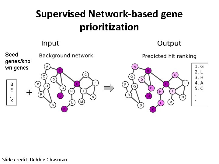
Supervised Network-based gene prioritization Seed genes/kno wn genes Slide credit: Debbie Chasman

Neighborhoods on graphs • Network-based methods rely on defining neighborhoods of genes • Neighborhoods of genes known for a disease can be used to prioritize additional genes • Local neighborhood – Immediate neighbor – Shortest path • Global neighborhood – Based on more global measures of distance between nodes • We have seen some ideas of neighborhoods on graphs in graph clustering

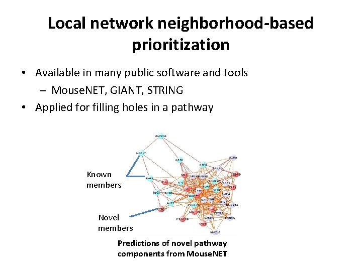
Local network neighborhood-based prioritization • Available in many public software and tools – Mouse. NET, GIANT, STRING • Applied for filling holes in a pathway Known members Novel members Predictions of novel pathway components from Mouse. NET

Global network neighborhood-based prioritization • Global network neighborhood-based methods make use of the entire graph to define the similarity between two genes • Given a graph connecting nodes, global similarity can be defined using – Random walk – Diffusion kernel – Laplacian kernel – Heat kernel

Goals for today • Gene prioritization – Supervised methods – Unsupervised methods • Gene. Wanderer: Walking the Interactome for Prioritization of Candidate Disease Genes – An example of supervised, graph diffusion-based approach • Other applications of random walks on graphs

Motivation of Gene. Wanderer • There are many diseases for which we do not know the causal genes • Previous approaches have used protein-protein interaction networks, but in a limited way – Only local similarity was used • Can we use global graph distance? • Does global distance help and improve current prioritization techniques? S. Köhler, S. Bauer, D. Horn, and P. N. Robinson, "Walking the interactome for prioritization of candidate disease genes. " American journal of human genetics, vol. 82, no. 4, pp. 949958, Apr. 2008. [Online]. Available: http: //dx. doi. org/10. 1016/j. ajhg. 2008. 02. 013

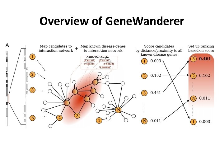
Overview of Gene. Wanderer

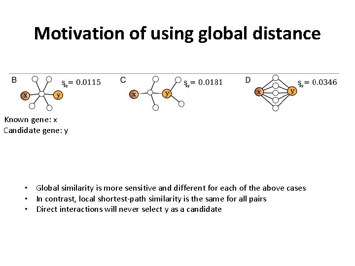
Motivation of using global distance Known gene: x Candidate gene: y • Global similarity is more sensitive and different for each of the above cases • In contrast, local shortest-path similarity is the same for all pairs • Direct interactions will never select y as a candidate

Global graph distances used in Gene. Wanderer • Random walk with restarts • Diffusion kernel

Random walk on graphs • A random walk is defined as a probabilistic traversal of a graph • At each time step, the walker transitions randomly to one of the neighbors of the current node. • Typically one can start anywhere on the graph • But one can put priors on the walk based on what we know about candidate genes. • The random walk converges to some distribution of the number of times a gene is visited. • The distribution can be used to rank genes

Random walk on graphs • Random walk on a graph requires us to define transition probabilities • Transition probability is obtained by dividing each entry by the row sum or column sum • One step of the random walk corresponds to one matrix multiplication of the transition matrix • Suppose we started at node a, what is the probability of reaching other nodes after t steps? • tth power of the transition matrix tell us the probability of reaching node j from node i after t steps on the random walk

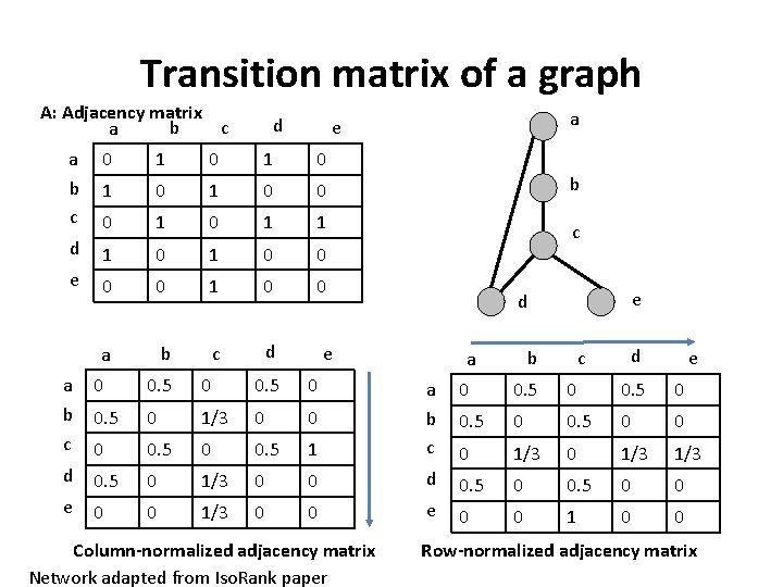
Transition matrix of a graph A: Adjacency matrix c b a d a e a b c 0 1 0 1 0 0 b 0 1 1 d 1 0 0 c e 0 0 1 0 0 a b c d e a b c 0 0. 5 0 1/3 0 0. 5 d 0. 5 0 1/3 e 0 0 1/3 e d d c b a e 0 0. 5 0 0 1 a b c 0 1/3 1/3 0 0 d 0. 5 0 0 0 0 e 0 0 1 0 0 Column-normalized adjacency matrix Network adapted from Iso. Rank paper Row-normalized adjacency matrix

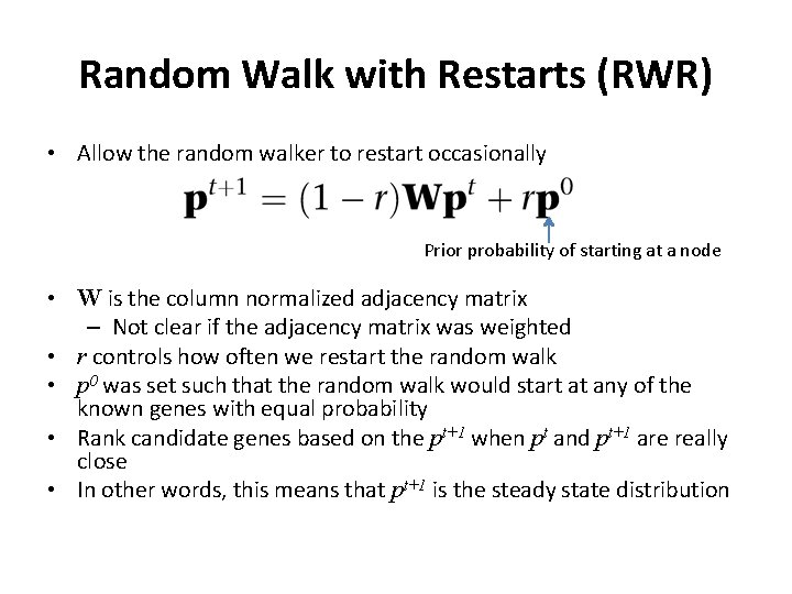
Random Walk with Restarts (RWR) • Allow the random walker to restart occasionally Prior probability of starting at a node • W is the column normalized adjacency matrix – Not clear if the adjacency matrix was weighted • r controls how often we restart the random walk • p 0 was set such that the random walk would start at any of the known genes with equal probability • Rank candidate genes based on the pt+1 when pt and pt+1 are really close • In other words, this means that pt+1 is the steady state distribution

RWR continued • Intuitively, this approach gives the probability of reaching a specific node, given that a random walk starts at a given node, while taking all intermediate paths into account • By making the random walk start from known disease genes we obtain a global proximity measure from these known genes

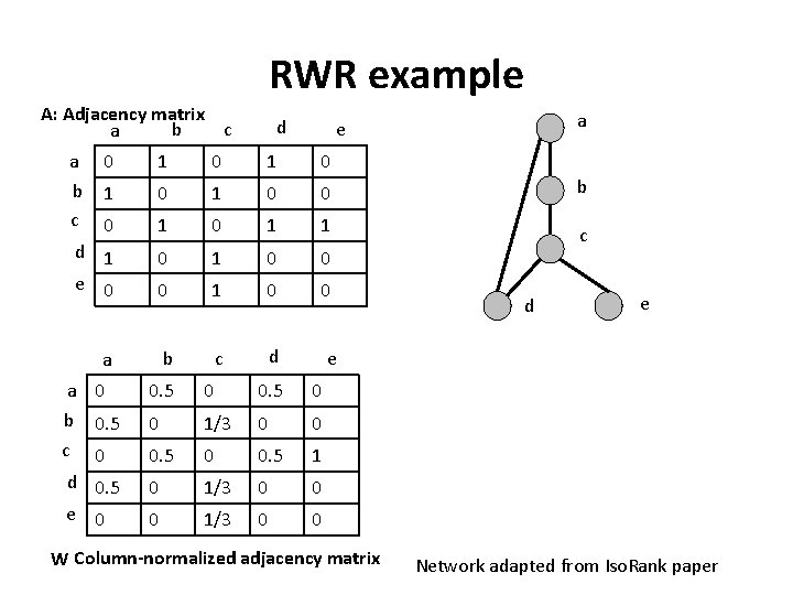
RWR example A: Adjacency matrix c b a d a e 0 1 0 1 0 0 b 0 1 1 d 1 e 0 0 1 0 0 c 0 1 0 0 b c d a b c a d e e a 0 b 0. 5 c 0 d 0. 5 0 0 1/3 0 0 0. 5 1 0 1/3 0 0 e 0 0 1/3 0 0 W Column-normalized adjacency matrix Network adapted from Iso. Rank paper

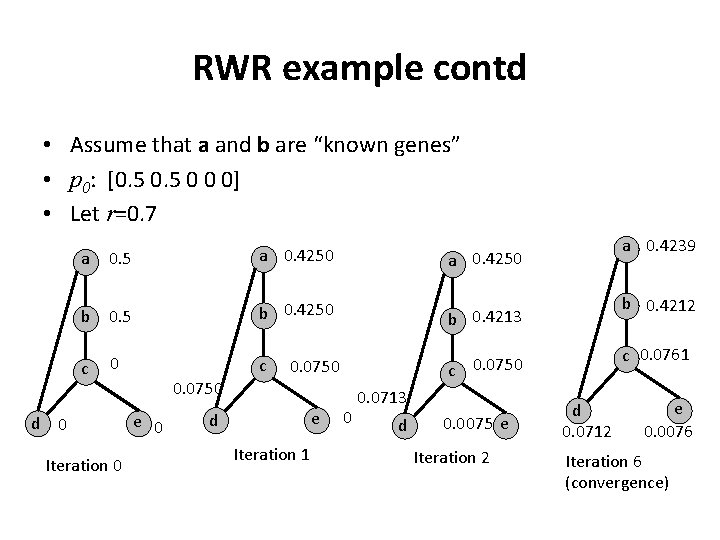
RWR example contd • Assume that a and b are “known genes” • p 0: [0. 5 0 0 0] • Let r=0. 7 0. 5 a 0. 4250 b 0. 5 b 0. 4250 b 0. 4213 c c 0. 0750 a c 0 d 0 Iteration 0 0. 0750 e 0 e d Iteration 1 0 0. 0713 d 0. 0075 e Iteration 2 a 0. 4239 b 0. 4212 c 0. 0761 d 0. 0712 e 0. 0076 Iteration 6 (convergence)

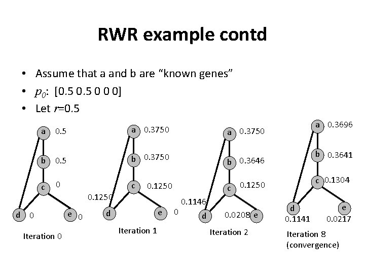
RWR example contd • Assume that a and b are “known genes” • p 0: [0. 5 0 0 0] • Let r=0. 5 a 0. 3750 b 0. 5 b 0. 3750 b 0. 3646 c c 0. 1250 a c 0 d 0 Iteration 0 0. 1250 e d Iteration 1 0 0. 1146 d 0. 0208 e Iteration 2 a 0. 3696 b 0. 3641 c 0. 1304 d 0. 1141 e 0. 0217 Iteration 8 (convergence)

Global graph distances used in Gene. Wanderer • Random walk with restarts • Diffusion kernel

Kernel • A Kernel k is a function that maps pairs of objects to a realvalued space • It enables one to define very general similarity functions between pairs of objects • Let denote a set of objects of a particular type – For example the set of images or a set of trees • A kernel k is defined as

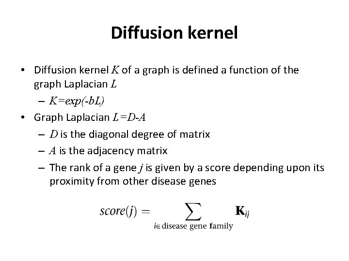
Diffusion kernel • Diffusion kernel K of a graph is defined a function of the graph Laplacian L – K=exp(-b. L) • Graph Laplacian L=D-A – D is the diagonal degree of matrix – A is the adjacency matrix – The rank of a gene j is given by a score depending upon its proximity from other disease genes

Diffusion kernel • The diffusion kernel gives a ranking of a new gene using the sum of a global distance measure from all known genes of a disease • Specifically the jth column corresponds to the stationary distribution of a random walk that started at node j.

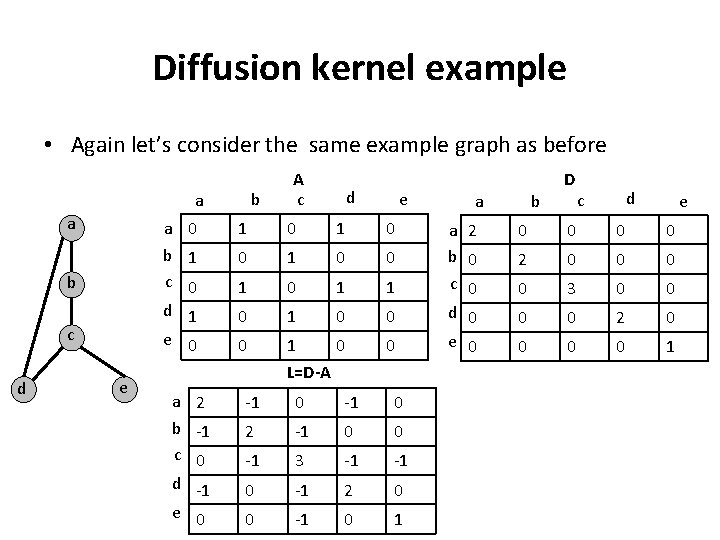
Diffusion kernel example • Again let’s consider the same example graph as before b a a b c d e A c d e a 0 b 1 c 0 d 1 1 0 0 1 0 1 1 0 e 0 0 1 0 b a D d c e 0 0 2 0 0 3 0 0 0 a 2 b 0 c 0 d 0 0 0 2 0 0 e 0 0 1 L=D-A a 2 b -1 c 0 d -1 -1 0 2 -1 0 0 -1 3 -1 -1 0 -1 2 0 e 0 0 -1 0 1

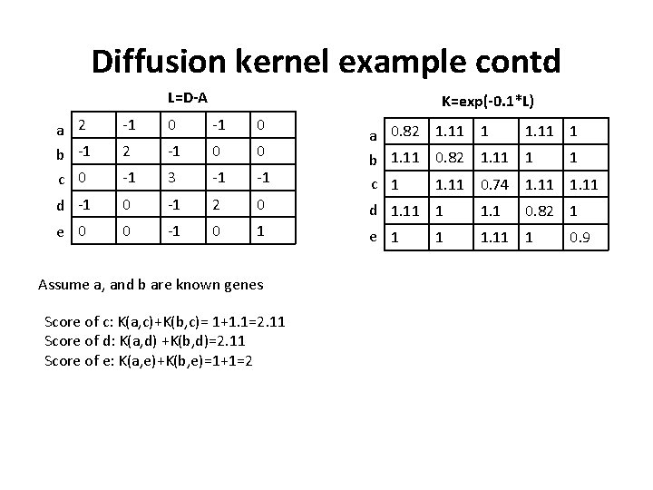
Diffusion kernel example contd L=D-A K=exp(-0. 1*L) a 2 b -1 c 0 -1 0 2 -1 0 0 -1 3 -1 -1 1. 11 1 a 0. 82 1. 11 1 1 b 1. 11 0. 82 1. 11 1 c 1 1. 11 0. 74 1. 11 d -1 0 -1 2 0 d 1. 11 1 1. 1 e 0 0 -1 0 1 e 1 1. 11 1 Assume a, and b are known genes Score of c: K(a, c)+K(b, c)= 1+1. 1=2. 11 Score of d: K(a, d) +K(b, d)=2. 11 Score of e: K(a, e)+K(b, e)=1+1=2 1 0. 82 1 0. 9

Competing methods • Direct interactions (DI) – A gene is predicted as a disease gene for disease j if it is a direct neighbor of a gene associated with a known gene of disease j • Shortest path (SP) – Rank gene based on the single shortest path to any known disease gene for disease j • ENDEAVOUR – Integrates gene expression, protein domain information, literature annotation – Based on an ensemble method, each component of the ensemble corresponds to a dataset • PROSPECTR – Sequence-based features using an alternating decision tree to output a likelihood of a gene to belong to a disease

Dataset • • Data source: – Online Mendelian Inheritance in Man (OMIM) • An Online Catalog of Human Genes and Genetic Disorders – Literature search to find genes clearly 110 different disease-gene families spanning different types of diseases: – 86 genetically heterogeneous disorders in which mutations in distinct genes are associated with similar or even indistinguishable phenotypes; – 12 cancer syndromes comprising genes associated with hereditary cancer, increased risk, or somatic mutation in a given cancer type; – 12 complex (polygenic) disorders that are known to be influenced by variation in multiple genes Total of 783 genes with 665 distinct genes – Some genes are associated with multiple diseases – Each family has 7 genes on average, largest family has 41 genes, smallest had 3 genes Interaction network of 35, 910 genes from human and 38, 975 from other organisms – Include experimentally verified and predicted interactions

Evaluation strategy • For each disease gene define an artificial linkage interval by selection 100 closest genes on the same chromosome • Evaluate performance based on leave one out for each disease gene family • Two assessment measures – An enrichment score: General idea is to compare the predicted rank to a rank obtained by random • Let grank be the rank of a particular gene • Enrichment score is defined as 50/grank • If a true disease gene is ranked the highest, it has an enrichment score of 50 • For all other genes, we have assigned a rank of 100. – Receiver Operator Curves (ROC) • Plot True Positive Rate (TPR) versus False Positive Rate (FPR) and compute Area Under the ROC (AUROC)

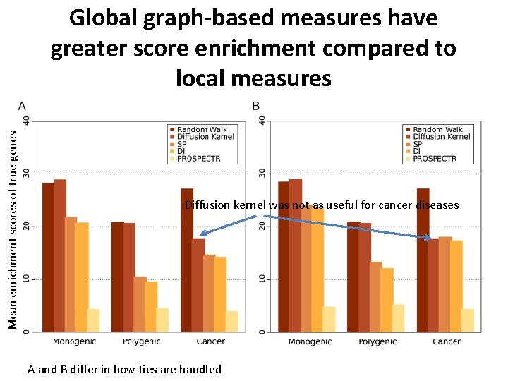
Mean enrichment scores of true genes Global graph-based measures have greater score enrichment compared to local measures Diffusion kernel was not as useful for cancer diseases A and B differ in how ties are handled

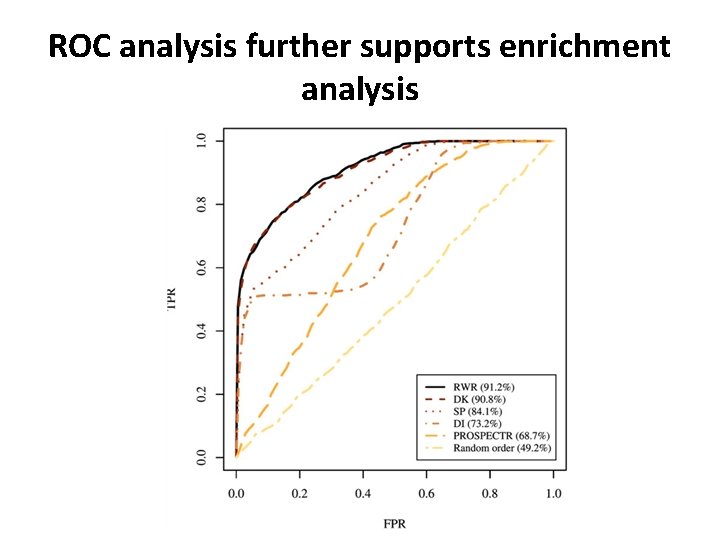
ROC analysis further supports enrichment analysis

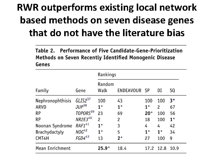
RWR outperforms existing local network based methods on seven disease genes that do not have the literature bias

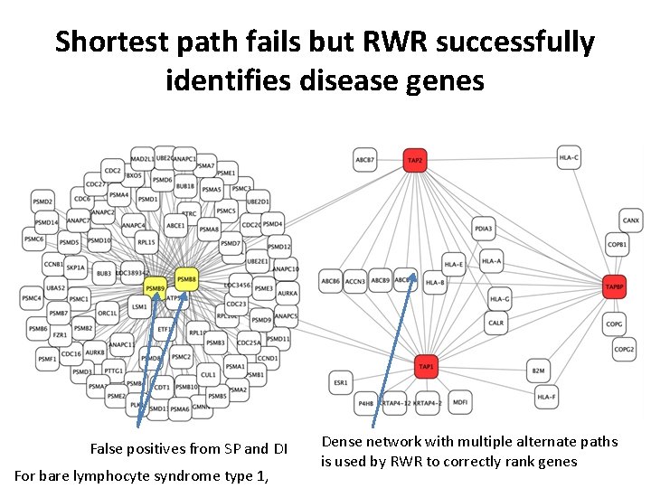
Shortest path fails but RWR successfully identifies disease genes False positives from SP and DI For bare lymphocyte syndrome type 1, Dense network with multiple alternate paths is used by RWR to correctly rank genes

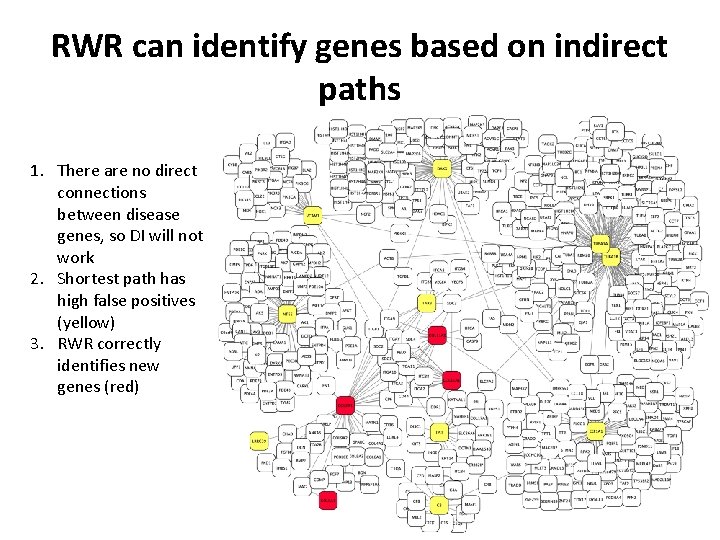
RWR can identify genes based on indirect paths 1. There are no direct connections between disease genes, so DI will not work 2. Shortest path has high false positives (yellow) 3. RWR correctly identifies new genes (red)

Summary of Gene. Wanderer results • Global similarity measured using both random walk and diffusion kernels are vastly superior than local distance measures • The authors generated a test set using a linkage based analysis – This is more realistic and similar to existing linkage-based approaches to find genes – Others have used a random set of test genes, which might not be correct because similar genes tend to cluster on chromosomes • How to define disease gene families? – This method needs known genes, although not many. Was shown to work for as small as 3 genes. – Existing approaches like ENDEAVOUR may not work

Concluding remarks • Phenotypically similar diseases likely represent perturbations to the same subnetwork or are topologically close. • This approach works for situations where there are some known genes that can be used to rank other genes with respect to them – But this may not be the case always. How to extend? • Current interaction networks are incomplete • Each disease was considered one at a time – Can we share information between diseases to better prioritize genes? • Recent approaches go beyond genes: prioritizing GWAS sequence variants (Net. WAS from GIANT http: //giant. princeton. edu )

Other applications of random walks • Hi-C matrix denoising • Single cell RNA-seq data denoising

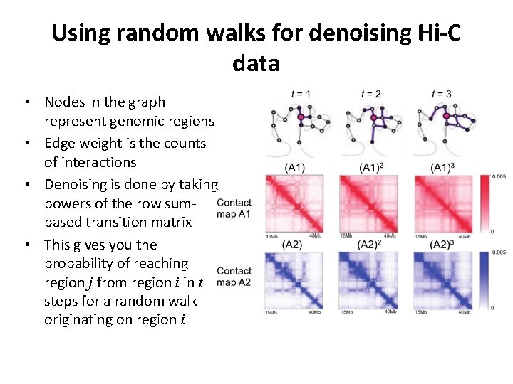
Using random walks for denoising Hi-C data • Nodes in the graph represent genomic regions • Edge weight is the counts of interactions • Denoising is done by taking powers of the row sumbased transition matrix • This gives you the probability of reaching region j from region i in t steps for a random walk originating on region i

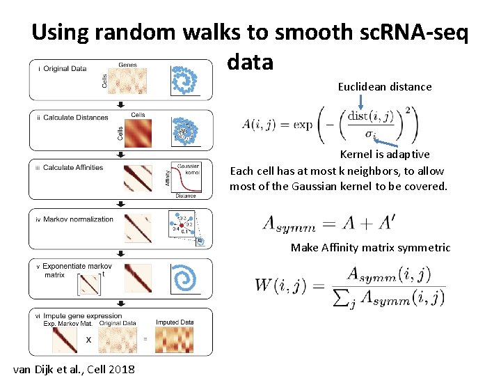
Using random walks to smooth sc. RNA-seq data Euclidean distance Kernel is adaptive Each cell has at most k neighbors, to allow most of the Gaussian kernel to be covered. Make Affinity matrix symmetric van Dijk et al. , Cell 2018

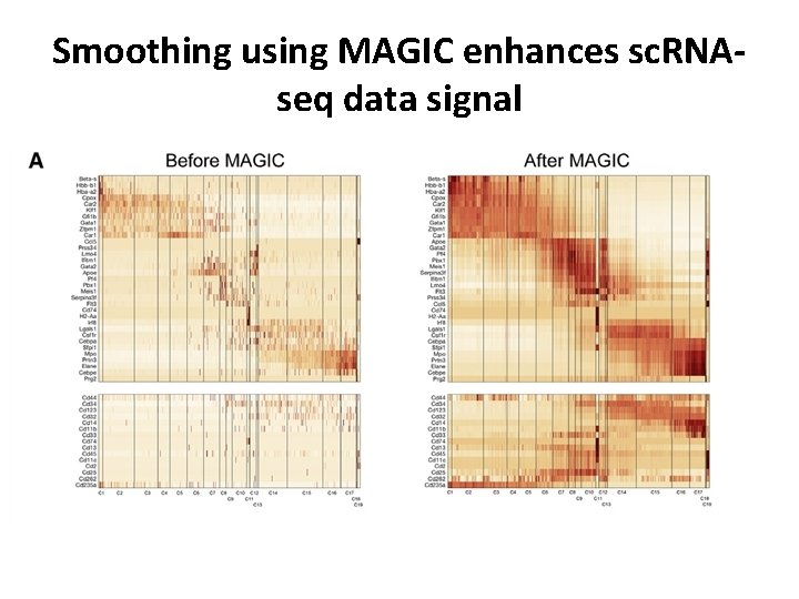
Smoothing using MAGIC enhances sc. RNAseq data signal