Graph Cuts Approach to the Problems of Image

Graph Cuts Approach to the Problems of Image Segmentation Based on presentations by: M Kummar – microsoft research Antong Chen Refael Vivanti
 = ∑ ci xi + ∑ cij xi(1 -xj) i i,")
Segmentation energy E(x) = ∑ ci xi + ∑ cij xi(1 -xj) i i, j E: {0, 1}n → R 0 → fg 1 → bg n = number of pixels Image (D)
 = ∑ ci xi + ∑ cij xi(1 -xj) i i,")
Segmentation energy E(x) = ∑ ci xi + ∑ cij xi(1 -xj) i i, j E: {0, 1}n → R 0 → fg 1 → bg n = number of pixels Unary Cost (ci) Dark (negative) Bright
 = ∑ ci xi + ∑ cij xi(1 -xj) i i,")
Segmentation energy E(x) = ∑ ci xi + ∑ cij xi(1 -xj) i i, j E: {0, 1}n → R 0 → fg 1 → bg n = number of pixels Discontinuity Cost (cij)
 = ∑ ci xi + ∑ cij xi(1 -xj) i i,")
Segmentation energy E(x) = ∑ ci xi + ∑ cij xi(1 -xj) i i, j E: {0, 1}n → R 0 → fg 1 → bg n = number of pixels x* = arg min E(x) x Global Minimum (x*) How to minimize E(x)?

The st-Mincut Problem Source 2 9 1 v 1 5 2 Sink v 2 4 Graph (V, E, C) Vertices V = {v 1, v 2. . . vn} Edges E = {(v 1, v 2). . } Costs C = {c(1, 2). . }

The st-Mincut Problem What is a st-cut? Source 2 9 1 v 1 5 2 Sink v 2 4
 divides the nodes")
The st-Mincut Problem What is a st-cut? An st-cut (S, T) divides the nodes between source and sink. Source 2 9 1 v 1 5 2 v 2 4 Sink 5 + 2 + 9 = 16 What is the cost of a st-cut? Sum of cost of all edges going from S to T
 divides the nodes")
The st-Mincut Problem What is a st-cut? An st-cut (S, T) divides the nodes between source and sink. Source 2 9 1 v 1 5 2 v 2 4 Sink 2 + 1 + 4 = 7 What is the cost of a st-cut? Sum of cost of all edges going from S to T What is the st-mincut? st-cut with the minimum cost

How to compute the st-mincut? Solve the dual maximum flow problem Compute the maximum flow between Source and Sink Source 2 9 1 v 1 5 2 Sink v 2 Constraints Edges: Flow < Capacity Nodes: Flow in = Flow out 4 Min-cutMax-flow Theorem In every network, the maximum flow equals the cost of the st-mincut

Maxflow Algorithms Flow = 0 Augmenting Path Based Algorithms Source 2 9 1 v 1 5 2 Sink v 2 4 1. Find path from source to sink with positive capacity 2. Push maximum possible flow through this path 3. Repeat until no path can be found Algorithms assume non-negative capacity

Maxflow Algorithms Flow = 0 Augmenting Path Based Algorithms Source 2 9 1 v 1 5 2 Sink v 2 4 1. Find path from source to sink with positive capacity 2. Push maximum possible flow through this path 3. Repeat until no path can be found Algorithms assume non-negative capacity

Maxflow Algorithms Flow = 0 + 2 Augmenting Path Based Algorithms Source 2 -2 9 1 v 1 2 5 -2 Sink v 2 4 1. Find path from source to sink with positive capacity 2. Push maximum possible flow through this path 3. Repeat until no path can be found Algorithms assume non-negative capacity

Maxflow Algorithms Flow = 2 Augmenting Path Based Algorithms Source 0 9 1 v 1 3 2 Sink v 2 4 1. Find path from source to sink with positive capacity 2. Push maximum possible flow through this path 3. Repeat until no path can be found Algorithms assume non-negative capacity

Maxflow Algorithms Flow = 2 Augmenting Path Based Algorithms Source 0 9 1 v 1 3 2 Sink v 2 4 1. Find path from source to sink with positive capacity 2. Push maximum possible flow through this path 3. Repeat until no path can be found Algorithms assume non-negative capacity

Maxflow Algorithms Flow = 2 Augmenting Path Based Algorithms Source 0 9 1 v 1 3 2 Sink v 2 4 1. Find path from source to sink with positive capacity 2. Push maximum possible flow through this path 3. Repeat until no path can be found Algorithms assume non-negative capacity

Maxflow Algorithms Flow = 2 + 4 Augmenting Path Based Algorithms Source 0 5 1 v 1 3 2 Sink v 2 0 1. Find path from source to sink with positive capacity 2. Push maximum possible flow through this path 3. Repeat until no path can be found Algorithms assume non-negative capacity

Maxflow Algorithms Flow = 6 Augmenting Path Based Algorithms Source 0 5 1 v 1 3 2 Sink v 2 0 1. Find path from source to sink with positive capacity 2. Push maximum possible flow through this path 3. Repeat until no path can be found Algorithms assume non-negative capacity

Maxflow Algorithms Flow = 6 Augmenting Path Based Algorithms Source 0 5 1 v 1 3 2 Sink v 2 0 1. Find path from source to sink with positive capacity 2. Push maximum possible flow through this path 3. Repeat until no path can be found Algorithms assume non-negative capacity

Maxflow Algorithms Flow = 6 + 1 Augmenting Path Based Algorithms Source 0 4 1 -1 v 1 2 2+1 Sink v 2 0 1. Find path from source to sink with positive capacity 2. Push maximum possible flow through this path 3. Repeat until no path can be found Algorithms assume non-negative capacity

Maxflow Algorithms Flow = 7 Augmenting Path Based Algorithms Source 0 4 0 v 1 2 3 Sink v 2 0 1. Find path from source to sink with positive capacity 2. Push maximum possible flow through this path 3. Repeat until no path can be found Algorithms assume non-negative capacity

Maxflow Algorithms Flow = 7 Augmenting Path Based Algorithms Source 0 4 0 v 1 2 3 Sink v 2 0 1. Find path from source to sink with positive capacity 2. Push maximum possible flow through this path 3. Repeat until no path can be found Algorithms assume non-negative capacity

History. Augmenting of Maxflow Algorithms n: nodes Path and Push# Relabel m: #edges U: maximum edge weight Algorithms assume nonnegative edge weights [Slide credit: Andrew

History. Augmenting of Maxflow Algorithms n: nodes Path and Push# Relabel m: #edges U: maximum edge weight Algorithms assume nonnegative edge weights [Slide credit: Andrew

Augmenting Path based Algorithms Ford Fulkerson: Choose any augmenting path Source 1000 a 1 1000 a 2 0 1000 Sink

Augmenting Path based Algorithms Ford Fulkerson: Choose any augmenting path Source 1000 a 1 1000 a 2 0 1000 Sink Bad Augmenting Paths

Augmenting Path based Algorithms Ford Fulkerson: Choose any augmenting path Source 1000 a 1 1000 a 2 0 1000 Sink Bad Augmenting Path

Augmenting Path based Algorithms Ford Fulkerson: Choose any augmenting path Source 999 a 1 1000 0 1000 a 2 1 999 Sink

Augmenting Path based Algorithms Ford Fulkerson: Choose any augmenting path Source 999 a 1 1000 0 1000 a 2 1 999 Sink We will have to perform 2000 augmentations! Worst case complexity: O (m x Total_Flow) (Pseudo-polynomial bound: depends on flow) n: #nodes m: #edges

Augmenting Path based Algorithms Dinic: Choose shortest augmenting path Source 1000 a 1 1000 a 2 0 1000 Sink Worst case Complexity: O (m n 2) n: #nodes m: #edges
")
St-mincut and Energy Minimization Functions of boolean variables E: {0, 1}n → R E(x) = ∑ ci xi + ∑ cij xi(1 -xj) i i, j cij≥ 0 Polynomial time st-mincut algorithms require non-negative edge weights

Constructing a Graph from an Image • Two kinds of vertices • Two kinds of edges • Cut - Segmentation

So how does this work? Construct a graph such that: 1. Any st-cut corresponds to an assignment of x 2. The cost of the cut is equal to the energy of x : E(x) S st-mincut E(x) T Solution
 Graph Construction Source (0) a 1 a 2 Sink (1)")
E(a 1, a 2) Graph Construction Source (0) a 1 a 2 Sink (1)
 = 2 a 1 2 1 Source (0)")
Graph Construction E(a , a ) = 2 a 1 2 1 Source (0) 2 a 1 a 2 Sink (1)
 = 2 a + 5ā 1 2 1")
Graph Construction E(a , a ) = 2 a + 5ā 1 2 1 1 Source (0) 2 a 1 a 2 5 Sink (1)
 = 2 a + 5ā + 9 a")
Graph Construction E(a , a ) = 2 a + 5ā + 9 a + 4ā 1 2 1 1 2 2 Source (0) 2 9 a 1 a 2 5 4 Sink (1)
 = 2 a + 5ā + 9 a")
Graph Construction E(a , a ) = 2 a + 5ā + 9 a + 4ā + 2 a ā 1 2 1 1 2 2 1 2 Source (0) 9 2 a 1 a 2 2 5 4 Sink (1)
 = 2 a + 5ā + 9 a")
Graph Construction E(a , a ) = 2 a + 5ā + 9 a + 4ā + 2 a ā + ā a 1 2 1 1 2 2 1 2 Source (0) 9 2 1 a 2 2 5 4 Sink (1) 1 2
 = 2 a 1 + 5ā1+ 9 a")
Graph Construction E(a 1, a 2) = 2 a 1 + 5ā1+ 9 a 2 + 4ā2 + 2 a 1ā2 + ā1 a 2 Source (0) 9 2 1 a 2 2 5 4 Sink (1)
 = 2 a 1 + 5ā1+ 9 a")
Graph Construction E(a 1, a 2) = 2 a 1 + 5ā1+ 9 a 2 + 4ā2 + 2 a 1ā2 + ā1 a 2 Source (0) 9 2 1 a 2 2 5 Cost of cut = 11 4 Sink (1) a 1 = 1 a 2 = 1 E (1, 1) = 11
 = 2 a 1 + 5ā1+ 9 a")
Graph Construction E(a 1, a 2) = 2 a 1 + 5ā1+ 9 a 2 + 4ā2 + 2 a 1ā2 + ā1 a 2 Source (0) 9 2 1 a 2 2 5 st-mincut cost = 8 4 Sink (1) a 1 = 1 a 2 = 0 E (1, 0) = 8

How does the code look like? Graph *g; For all pixels p /* Add a node to the graph */ node. ID(p) = g->add_node(); Source (0) /* Set cost of terminal edges */ set_weights(node. ID(p), fg. Cost(p), bg. Cost(p)); end for all adjacent pixels p, q add_weights(node. ID(p), node. ID(q), cost); end g->compute_maxflow(); label_p = g->is_connected_to_source(node. ID(p)); // is the label of pixel p (0 or 1) Sink (1)
")
How does the code look like? Graph *g; For all pixels p Source (0) /* Add a node to the graph */ node. ID(p) = g->add_node(); /* Set cost of terminal edges */ set_weights(node. ID(p), fg. Cost(p), bg. Cost(p)); end for all adjacent pixels p, q add_weights(node. ID(p), node. ID(q), cost); end g->compute_maxflow(); label_p = g->is_connected_to_source(node. ID(p)); // is the label of pixel p (0 or 1) bg. Cost(a 1) a 1 fg. Cost(a 1) bg. Cost(a 2) a 2 fg. Cost(a 2) Sink (1)
")
How does the code look like? Graph *g; For all pixels p Source (0) /* Add a node to the graph */ node. ID(p) = g->add_node(); /* Set cost of terminal edges */ set_weights(node. ID(p), fg. Cost(p), bg. Cost(p)); end for all adjacent pixels p, q add_weights(node. ID(p), node. ID(q), cost(p, q)); end g->compute_maxflow(); label_p = g->is_connected_to_source(node. ID(p)); // is the label of pixel p (0 or 1) bg. Cost(a 2) bg. Cost(a 1) cost(p, a 1 a 2 q) fg. Cost(a 1) fg. Cost(a 2) Sink (1)
")
How does the code look like? Graph *g; For all pixels p Source (0) /* Add a node to the graph */ node. ID(p) = g->add_node(); /* Set cost of terminal edges */ set_weights(node. ID(p), fg. Cost(p), bg. Cost(p)); end for all adjacent pixels p, q add_weights(node. ID(p), node. ID(q), cost(p, q)); end g->compute_maxflow(); label_p = g->is_connected_to_source(node. ID(p)); bg. Cost(a 2) bg. Cost(a 1) cost(p, a 1 a 2 q) fg. Cost(a 1) fg. Cost(a 2) Sink (1) // is the label of pixel p (0 or 1) a 1 = bg a 2 = fg

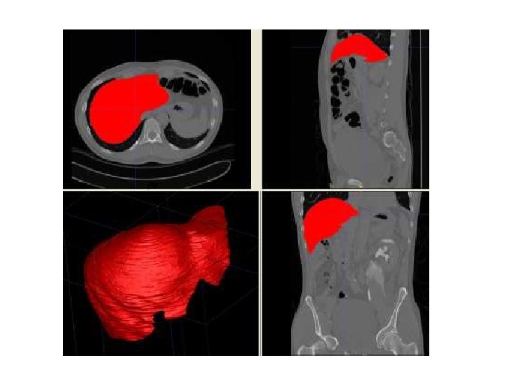
results של ריאה CT
- Slides: 50