Graph Clustering Why graph clustering is useful Distance

Graph Clustering

Why graph clustering is useful? • Distance matrices are graphs as useful as any other clustering • Identification of communities in social networks • Webpage clustering for better data management of web data

Outline • • • Min s-t cut problem Min cut problem Multiway cut Minimum k-cut Other normalized cuts and spectral graph partitionings

Min s-t cut • Weighted graph G(V, E) • An s-t cut C = (S, T) of a graph G = (V, E) is a cut partition of V into S and T such that s∈S and t∈T • Cost of a cut: Cost(C) = Σe(u, v) uЄS, v ЄT w(e) • Problem: Given G, s and t find the minimum cost s-t cut

Max flow problem • Flow network – Abstraction for material flowing through the edges – G = (V, E) directed graph with no parallel edges – Two distinguished nodes: s = source, t= sink – c(e) = capacity of edge e

Cuts • An s-t cut is a partition (S, T) of V with sЄS and tЄT • capacity of a cut (S, T) is cap(S, T) = Σe out of Sc(e) • Find s-t cut with the minimum capacity: this problem can be solved optimally in polynomial time by using flow techniques

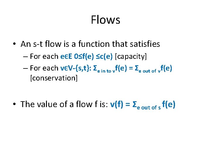
Flows • An s-t flow is a function that satisfies – For each eЄE 0≤f(e) ≤c(e) [capacity] – For each vЄV-{s, t}: Σe in to vf(e) = Σe out of vf(e) [conservation] • The value of a flow f is: v(f) = Σe out of s f(e)

Max flow problem • Find s-t flow of maximum value

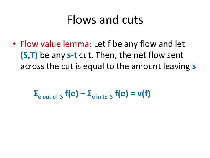
Flows and cuts • Flow value lemma: Let f be any flow and let (S, T) be any s-t cut. Then, the net flow sent across the cut is equal to the amount leaving s Σe out of S f(e) – Σe in to S f(e) = v(f)

Flows and cuts • Weak duality: Let f be any flow and let (S, T) be any s-t cut. Then the value of the flow is at most the capacity of the cut defined by (S, T): v(f) ≤cap(S, T)

Certificate of optimality • Let f be any flow and let (S, T) be any cut. If v(f) = cap(S, T) then f is a max flow and (S, T) is a min cut. • The min-cut max-flow problems can be solved optimally in polynomial time!

Setting • Connected, undirected graph G=(V, E) • Assignment of weights to edges: w: E R+ • Cut: Partition of V into two sets: V’, V-V’. The set of edges with one end point in V and the other in V’ define the cut • The removal of the cut disconnects G • Cost of a cut: sum of the weights of the edges that have one of their end point in V’ and the other in V-V’

Min cut problem • Can we solve the min-cut problem using an algorithm for s-t cut?

Randomized min-cut algorithm • Repeat : pick an edge uniformly at random and merge the two vertices at its end-points – If as a result there are several edges between some pairs of (newly-formed) vertices retain them all – Edges between vertices that are merged are removed (no selfloops) • Until only two vertices remain • The set of edges between these two vertices is a cut in G and is output as a candidate min-cut

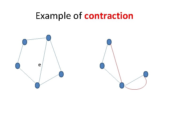
Example of contraction e

Observations on the algorithm • Every cut in the graph at any intermediate stage is a cut in the original graph

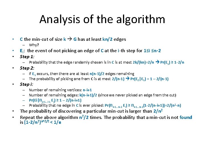
Analysis of the algorithm • C the min-cut of size k G has at least kn/2 edges – Why? • • Ei: the event of not picking an edge of C at the i-th step for 1≤i ≤n-2 Step 1: – Probability that the edge randomly chosen is in C is at most 2 k/(kn)=2/n Pr(E 1) ≥ 1 -2/n Step 2: – If E 1 occurs, then there at least n(n-1)/2 edges remaining – The probability of picking one from C is at most 2/(n-1) Pr(E 2|E 1) = 1 – 2/(n-1) Step i: – – • • Number of remaining vertices: n-i+1 Number of remaining edges: k(n-i+1)/2 (since we never picked an edge from the cut) Pr(Ei|Πj=1…i-1 Ej) ≥ 1 – 2/(n-i+1) Probability that no edge in C is ever picked: Pr(Πi=1…n-2 Ei) ≥ Πi=1…n-2(1 -2/(n-i+1))=2/(n 2 -n) The probability of discovering a particular min-cut is larger than 2/n 2 Repeat the above algorithm n 2/2 times. The probability that a min-cut is not found is (1 -2/n 2)n^2/2 < 1/e

Multiway cut (analogue of s-t cut) • Problem: Given a set of terminals S = {s 1, …, sk} subset of V, a multiway cut is a set of edges whose removal disconnects the terminals from each other. The multiway cut problem asks for the minimum weight such set. • The multiway cut problem is NP-hard (for k>2)

Algorithm for multiway cut • For each i=1, …, k, compute the minimum weight isolating cut for si, say Ci • Discard the heaviest of these cuts and output the union of the rest, say C • Isolating cut for si: The set of edges whose removal disconnects si from the rest of the terminals • How can we find a minimum-weight isolating cut?

Approximation result • The previous algorithm achieves an approximation guarantee of 2 -2/k • Proof

Minimum k-cut • A set of edges whose removal leaves k connected components is called a k-cut. The minimum k-cut problem asks for a minimum-weight k-cut • Recursively compute cuts in G (and the resulting connected components) until there are k components left • This is a (2 -2/k)-approximation algorithm

Minimum k-cut algorithm • Compute the Gomory-Hu tree T for G • Output the union of the lightest k-1 cuts of the n-1 cuts associated with edges of T in G; let C be this union • The above algorithm is a (2 -2/k)approximation algorithm

Gomory-Hu Tree • T is a tree with vertex set V • The edges of T need not be in E • Let e be an edge in T; its removal from T creates two connected components with vertex sets (S, S’) • The cut in G defined by partition (S, S’) is the cut associated with e in G

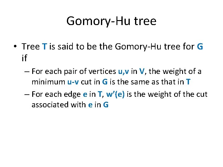
Gomory-Hu tree • Tree T is said to be the Gomory-Hu tree for G if – For each pair of vertices u, v in V, the weight of a minimum u-v cut in G is the same as that in T – For each edge e in T, w’(e) is the weight of the cut associated with e in G

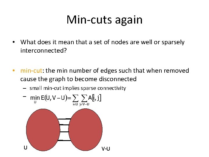
Min-cuts again • What does it mean that a set of nodes are well or sparsely interconnected? • min-cut: the min number of edges such that when removed cause the graph to become disconnected – small min-cut implies sparse connectivity – U V-U

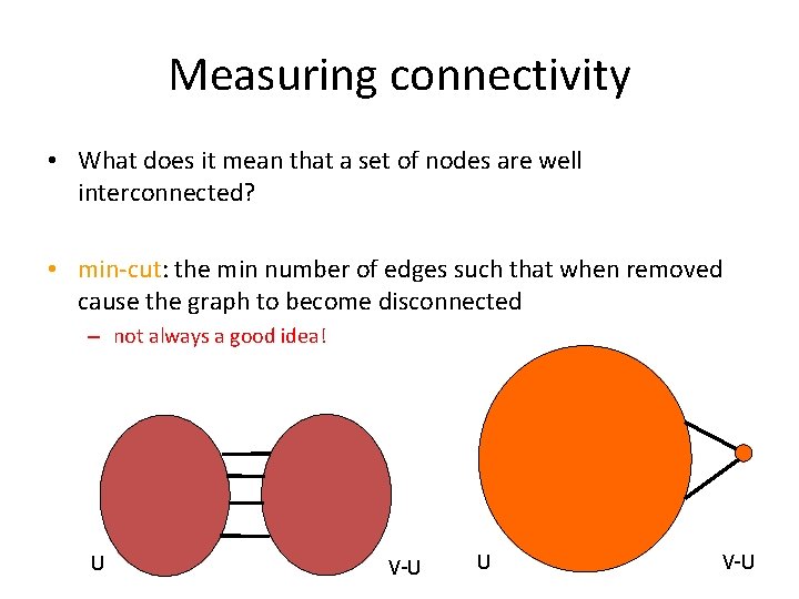
Measuring connectivity • What does it mean that a set of nodes are well interconnected? • min-cut: the min number of edges such that when removed cause the graph to become disconnected – not always a good idea! U V-U

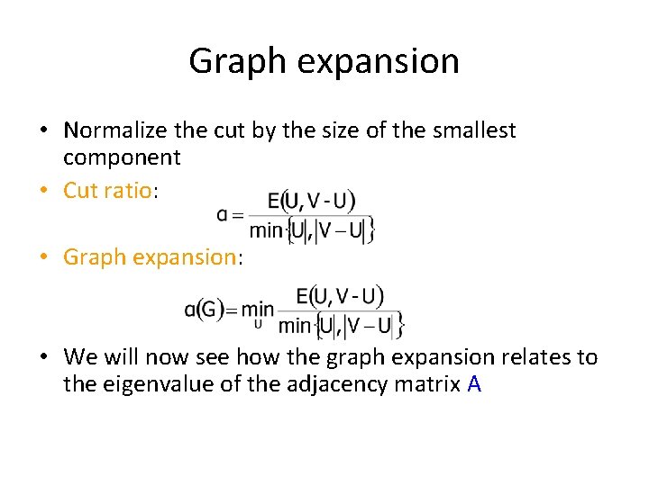
Graph expansion • Normalize the cut by the size of the smallest component • Cut ratio: • Graph expansion: • We will now see how the graph expansion relates to the eigenvalue of the adjacency matrix A

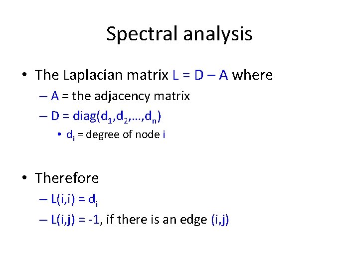
Spectral analysis • The Laplacian matrix L = D – A where – A = the adjacency matrix – D = diag(d 1, d 2, …, dn) • di = degree of node i • Therefore – L(i, i) = di – L(i, j) = -1, if there is an edge (i, j)

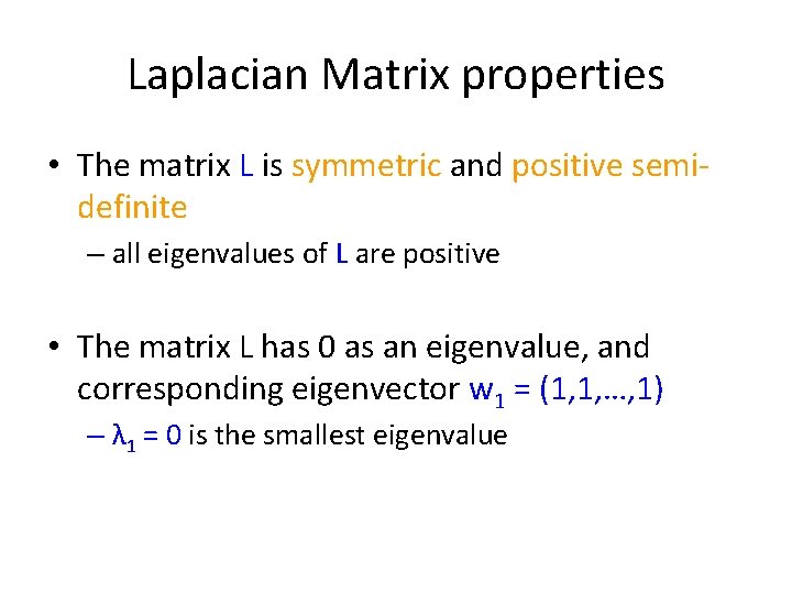
Laplacian Matrix properties • The matrix L is symmetric and positive semidefinite – all eigenvalues of L are positive • The matrix L has 0 as an eigenvalue, and corresponding eigenvector w 1 = (1, 1, …, 1) – λ 1 = 0 is the smallest eigenvalue

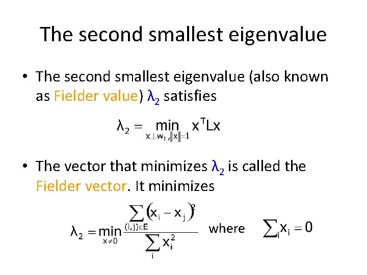
The second smallest eigenvalue • The second smallest eigenvalue (also known as Fielder value) λ 2 satisfies • The vector that minimizes λ 2 is called the Fielder vector. It minimizes where

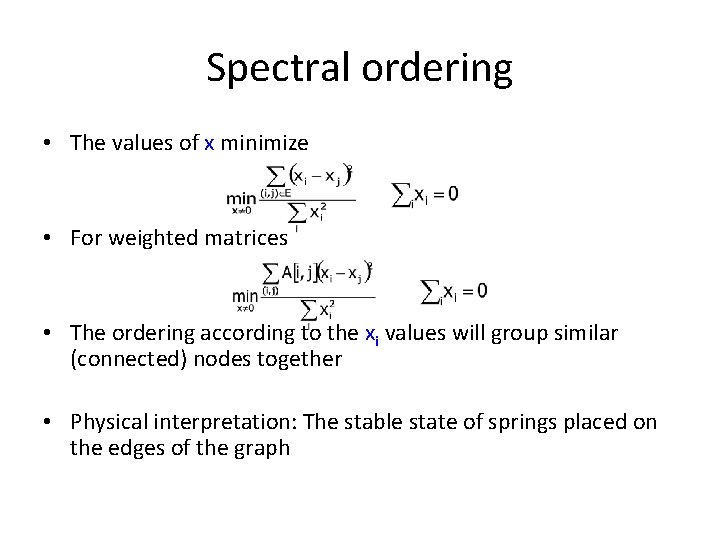
Spectral ordering • The values of x minimize • For weighted matrices • The ordering according to the xi values will group similar (connected) nodes together • Physical interpretation: The stable state of springs placed on the edges of the graph

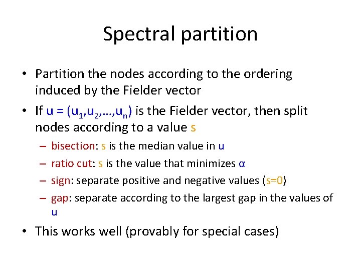
Spectral partition • Partition the nodes according to the ordering induced by the Fielder vector • If u = (u 1, u 2, …, un) is the Fielder vector, then split nodes according to a value s – – bisection: s is the median value in u ratio cut: s is the value that minimizes α sign: separate positive and negative values (s=0) gap: separate according to the largest gap in the values of u • This works well (provably for special cases)

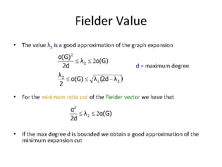
Fielder Value • The value λ 2 is a good approximation of the graph expansion d = maximum degree • For the minimum ratio cut of the Fielder vector we have that • If the max degree d is bounded we obtain a good approximation of the minimum expansion cut

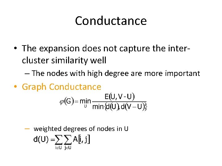
Conductance • The expansion does not capture the intercluster similarity well – The nodes with high degree are more important • Graph Conductance – weighted degrees of nodes in U

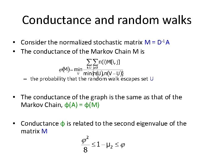
Conductance and random walks • Consider the normalized stochastic matrix M = D-1 A • The conductance of the Markov Chain M is – the probability that the random walk escapes set U • The conductance of the graph is the same as that of the Markov Chain, φ(A) = φ(M) • Conductance φ is related to the second eigenvalue of the matrix M

Interpretation of conductance • Low conductance means that there is some bottleneck in the graph – a subset of nodes not well connected with the rest of the graph. • High conductance means that the graph is well connected

Clustering Conductance • The conductance of a clustering is defined as the minimum conductance over all clusters in the clustering. • Maximizing conductance of clustering seems like a natural choice • …but it does not handle well outliers

A clustering bi-criterion • Maximize the conductance, but at the same time minimize the inter-cluster (between clusters) edges • A clustering C = {C 1, C 2, …, Cn} is a (c, e)clustering if – The conductance of each Ci is at least c – The total number of inter-cluster edges is at most a fraction e of the total edges

The clustering problem • Problem 1: Given c, find a (c, e)-clustering that minimizes e • Problem 2: Given e, find a (c, e)-clustering that maximizes c • Both problems are NP-hard

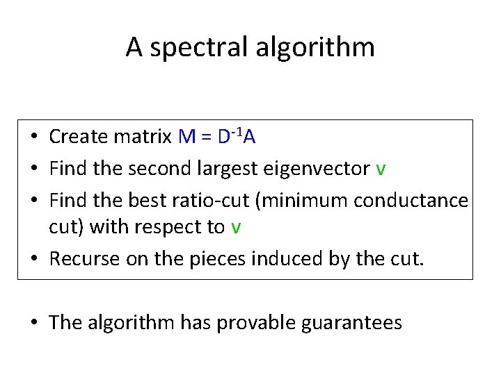
A spectral algorithm • Create matrix M = D-1 A • Find the second largest eigenvector v • Find the best ratio-cut (minimum conductance cut) with respect to v • Recurse on the pieces induced by the cut. • The algorithm has provable guarantees

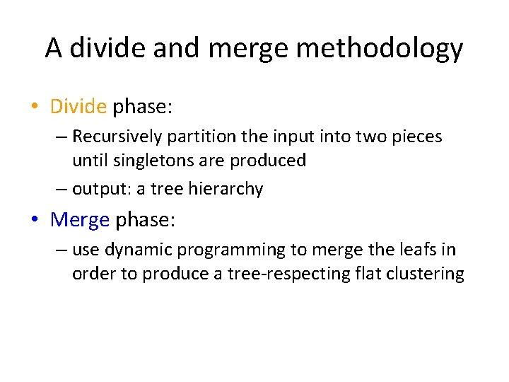
A divide and merge methodology • Divide phase: – Recursively partition the input into two pieces until singletons are produced – output: a tree hierarchy • Merge phase: – use dynamic programming to merge the leafs in order to produce a tree-respecting flat clustering

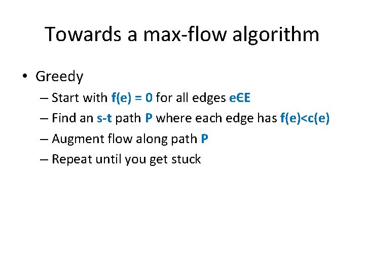
Towards a max-flow algorithm • Greedy – Start with f(e) = 0 for all edges eЄE – Find an s-t path P where each edge has f(e)<c(e) – Augment flow along path P – Repeat until you get stuck

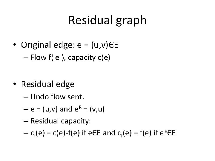
Residual graph • Original edge: e = (u, v)ЄE – Flow f( e ), capacity c(e) • Residual edge – Undo flow sent. – e = (u, v) and e. R = (v, u) – Residual capacity: – cf(e) = c(e)-f(e) if eЄE and cf(e) = f(e) if e. RЄE

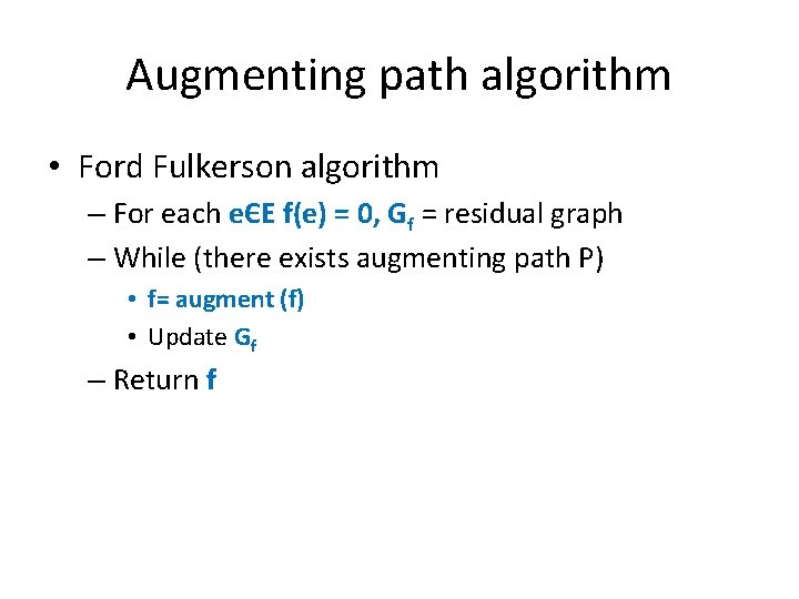
Augmenting path algorithm • Ford Fulkerson algorithm – For each eЄE f(e) = 0, Gf = residual graph – While (there exists augmenting path P) • f= augment (f) • Update Gf – Return f