Graph Algorithms in the Language of Linear Algebra

Graph Algorithms in the Language of Linear Algebra: How did we get here, where do we go next? John R. Gilbert University of California, Santa Barbara IPDPS Graph Algorithms Building Blocks May 21, 2018 1 Support: Intel, Microsoft, DOE Office of Science, NSF

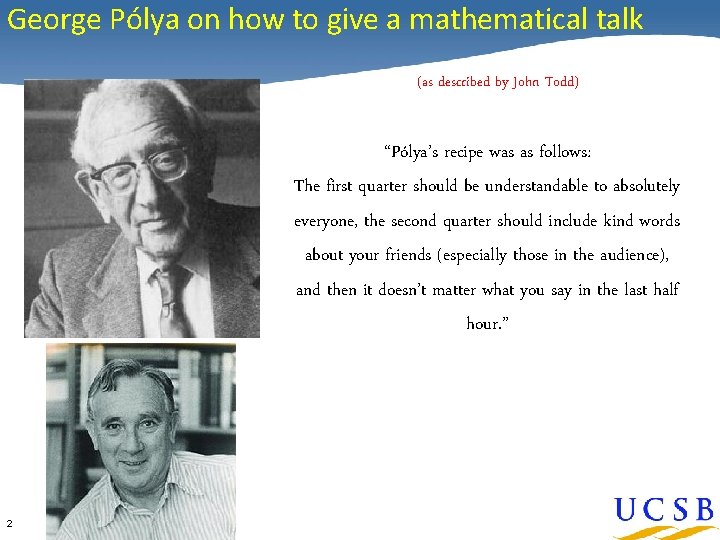
George Pólya on how to give a mathematical talk (as described by John Todd) “Pólya’s recipe was as follows: The first quarter should be understandable to absolutely everyone, the second quarter should include kind words about your friends (especially those in the audience), and then it doesn’t matter what you say in the last half hour. ” 2

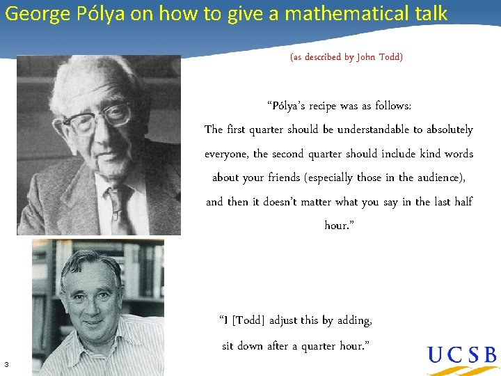
George Pólya on how to give a mathematical talk (as described by John Todd) “Pólya’s recipe was as follows: The first quarter should be understandable to absolutely everyone, the second quarter should include kind words about your friends (especially those in the audience), and then it doesn’t matter what you say in the last half hour. ” “I [Todd] adjust this by adding, 3 sit down after a quarter hour. ”

Prehistory In the year 1961. . . 4

Prehistory: A 1 -person game on graphs [S. Parter 1961] 5

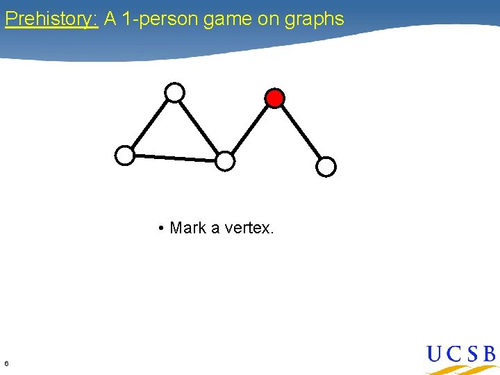
Prehistory: A 1 -person game on graphs • Mark a vertex. 6

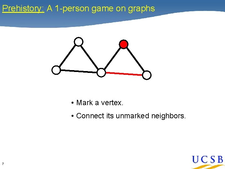
Prehistory: A 1 -person game on graphs • Mark a vertex. • Connect its unmarked neighbors. 7

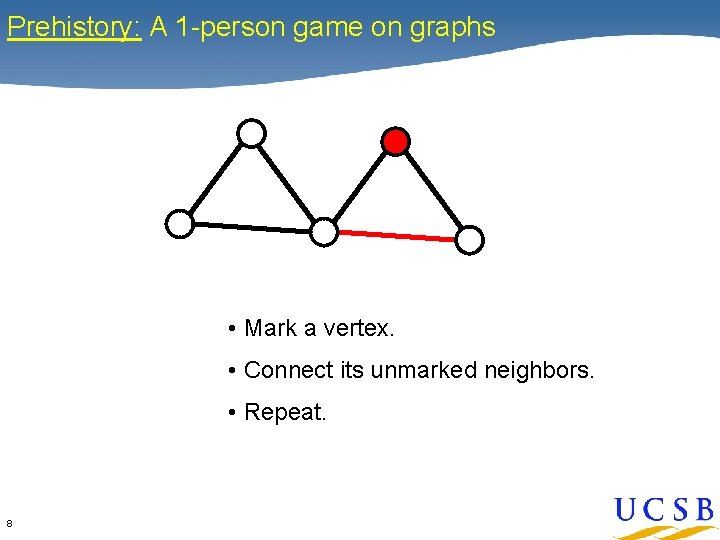
Prehistory: A 1 -person game on graphs • Mark a vertex. • Connect its unmarked neighbors. • Repeat. 8

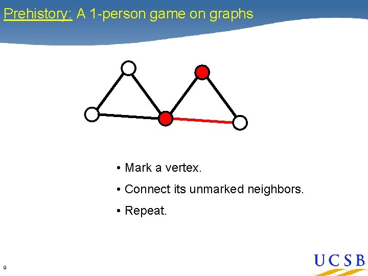
Prehistory: A 1 -person game on graphs • Mark a vertex. • Connect its unmarked neighbors. • Repeat. 9

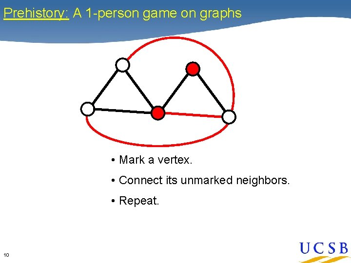
Prehistory: A 1 -person game on graphs • Mark a vertex. • Connect its unmarked neighbors. • Repeat. 10

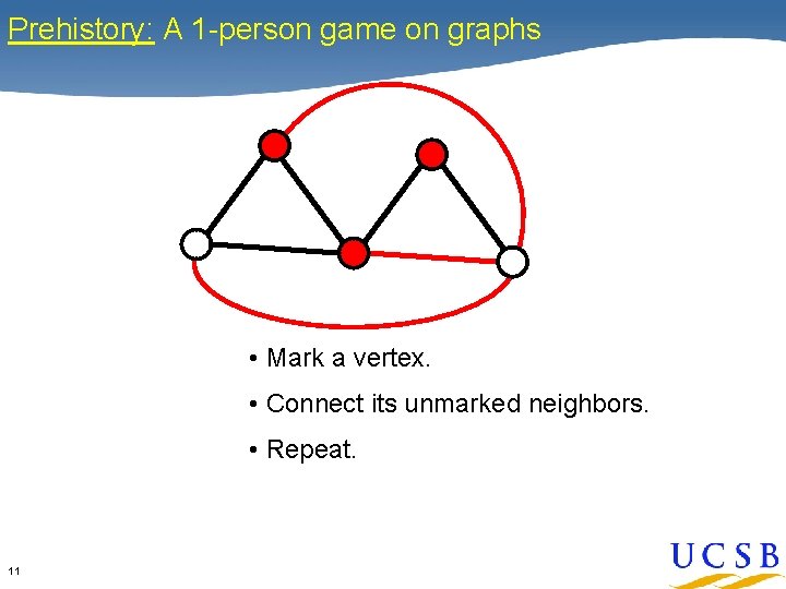
Prehistory: A 1 -person game on graphs • Mark a vertex. • Connect its unmarked neighbors. • Repeat. 11

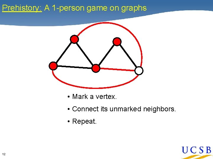
Prehistory: A 1 -person game on graphs • Mark a vertex. • Connect its unmarked neighbors. • Repeat. 12

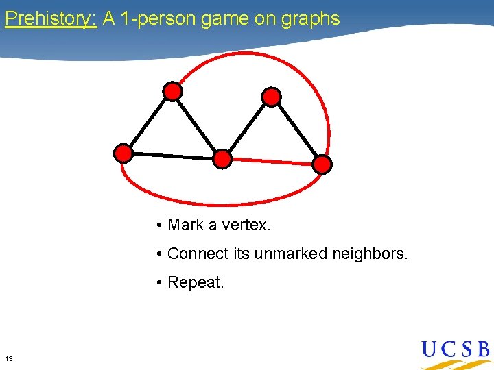
Prehistory: A 1 -person game on graphs • Mark a vertex. • Connect its unmarked neighbors. • Repeat. 13

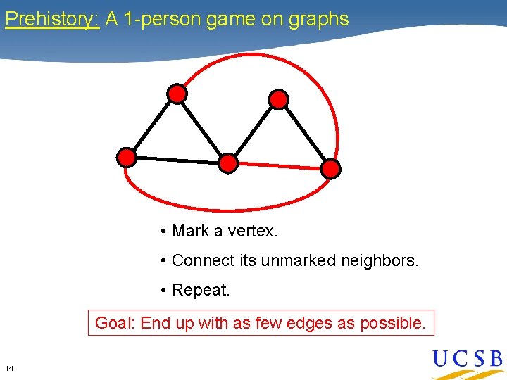
Prehistory: A 1 -person game on graphs • Mark a vertex. • Connect its unmarked neighbors. • Repeat. Goal: End up with as few edges as possible. 14

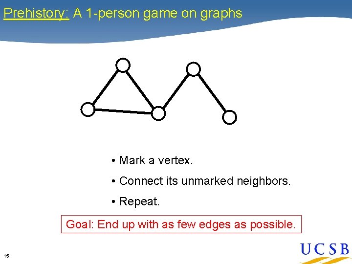
Prehistory: A 1 -person game on graphs • Mark a vertex. • Connect its unmarked neighbors. • Repeat. Goal: End up with as few edges as possible. 15

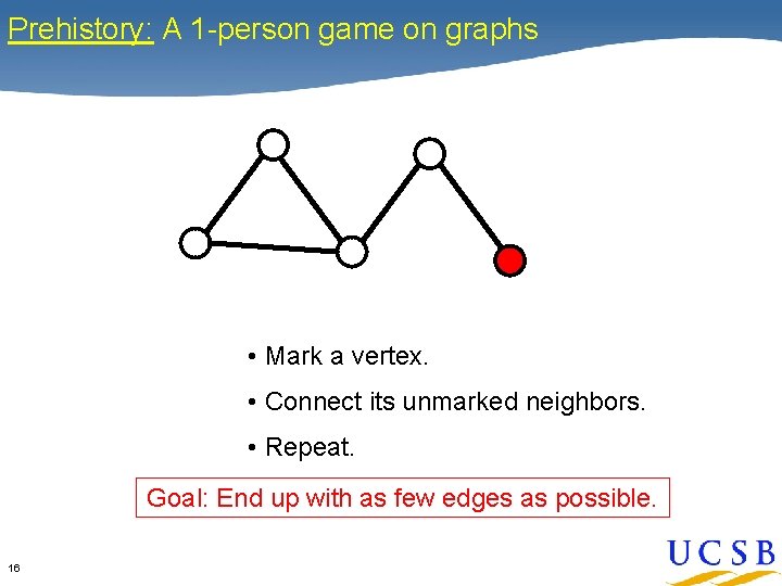
Prehistory: A 1 -person game on graphs • Mark a vertex. • Connect its unmarked neighbors. • Repeat. Goal: End up with as few edges as possible. 16

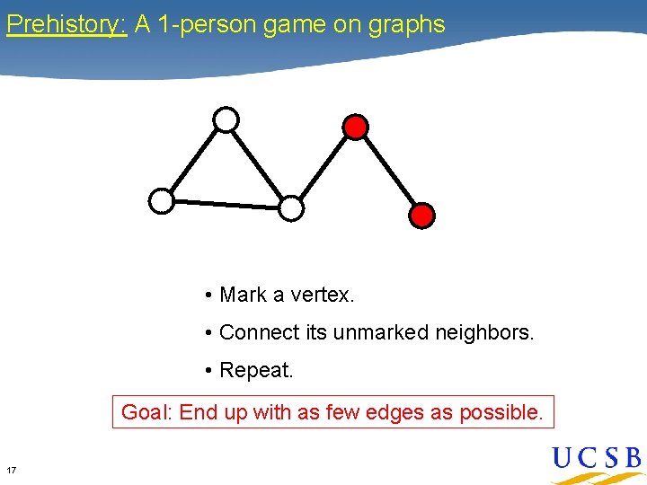
Prehistory: A 1 -person game on graphs • Mark a vertex. • Connect its unmarked neighbors. • Repeat. Goal: End up with as few edges as possible. 17

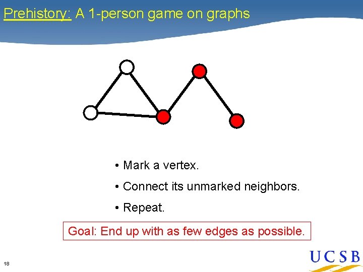
Prehistory: A 1 -person game on graphs • Mark a vertex. • Connect its unmarked neighbors. • Repeat. Goal: End up with as few edges as possible. 18

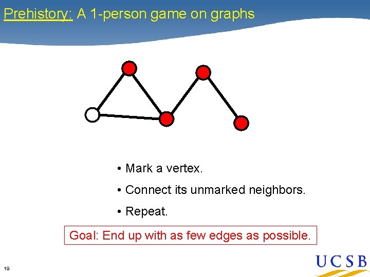
Prehistory: A 1 -person game on graphs • Mark a vertex. • Connect its unmarked neighbors. • Repeat. Goal: End up with as few edges as possible. 19

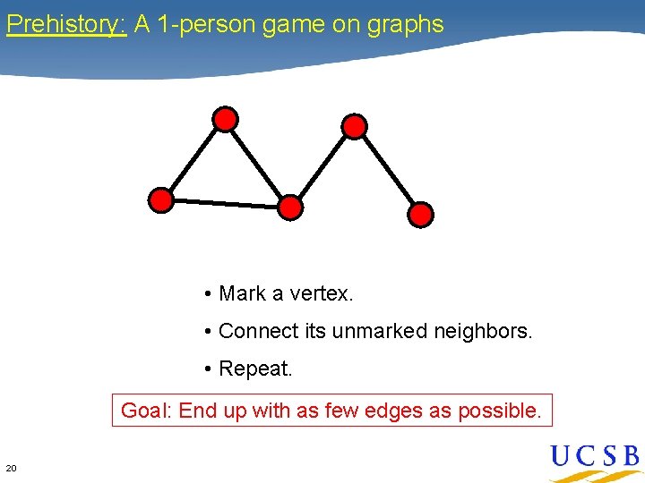
Prehistory: A 1 -person game on graphs • Mark a vertex. • Connect its unmarked neighbors. • Repeat. Goal: End up with as few edges as possible. 20

Vertex elimination game (or chordal completion) [Parter, Rose] Repeat: Choose a vertex v and mark it; Add edges between unmarked neighbors of v; Until: Every vertex is marked Goal: End up with as few edges as possible. 21 • Best play is NP-complete [Yannakakis 1981] • The final graph is always chordal (every cycle has a shortcut edge). • Perfect play is possible iff the initial graph is chordal. • Changing “fewest edges” to “smallest complete subgraph” gives the graph’s treewidth, which shows up in lots of graph algorithms.

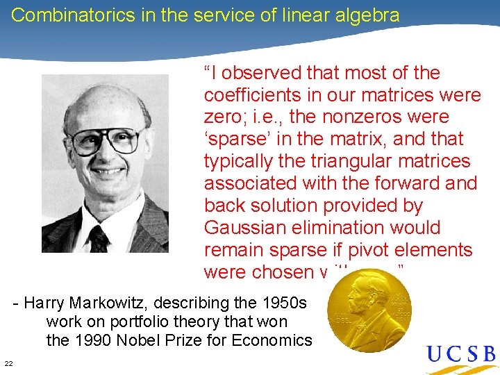
Combinatorics in the service of linear algebra “I observed that most of the coefficients in our matrices were zero; i. e. , the nonzeros were ‘sparse’ in the matrix, and that typically the triangular matrices associated with the forward and back solution provided by Gaussian elimination would remain sparse if pivot elements were chosen with care” - Harry Markowitz, describing the 1950 s work on portfolio theory that won the 1990 Nobel Prize for Economics 22

Cholesky factorization: A = LLT [Parter, Rose] Fill: new nonzeros in factor 3 1 7 Symmetric Gaussian elimination: 6 8 4 9 G(A) 23 4 10 5 2 6 8 9 10 5 G+(A) [chordal] 2 for j = 1 to n add edges between j’s higher-numbered neighbors

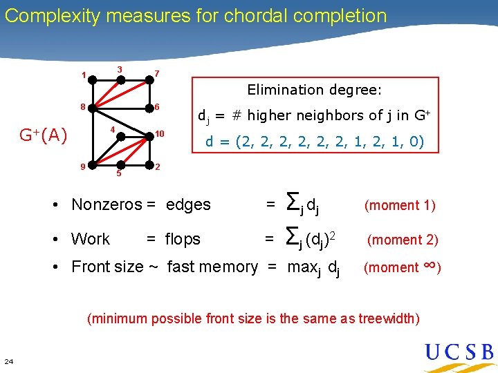
Complexity measures for chordal completion 3 1 7 Elimination degree: 6 8 G+(A) 4 9 dj = # higher neighbors of j in G+ 10 5 d = (2, 2, 2, 1, 0) 2 • Nonzeros = edges = • Work = = flops Σ j dj Σj (dj)2 • Front size ~ fast memory = maxj dj (moment 1) (moment 2) (moment ∞) (minimum possible front size is the same as treewidth) 24

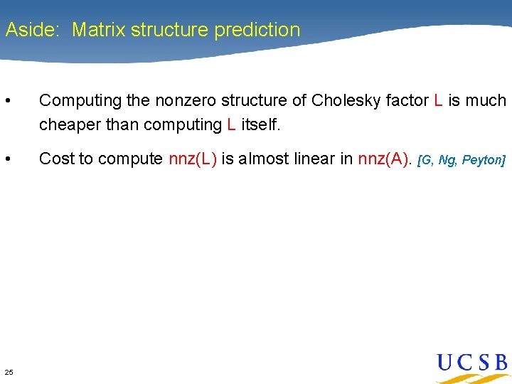
Aside: Matrix structure prediction • Computing the nonzero structure of Cholesky factor L is much cheaper than computing L itself. • Cost to compute nnz(L) is almost linear in nnz(A). [G, Ng, Peyton] Not so for sparse matrix product (Sp. GEMM); computing nnz(B*C) seems to be as hard as computing B*C. Can estimate nnz(B*C) accurately in time linear in nnz(B, C)! [E. Cohen 1998] Lots of cool recent work on sampling algorithms to estimate statistics of matrix functions. 25

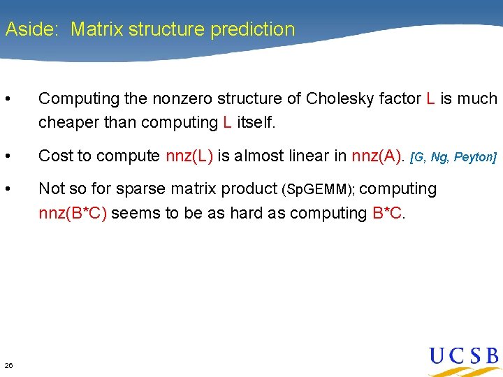
Aside: Matrix structure prediction • Computing the nonzero structure of Cholesky factor L is much cheaper than computing L itself. • Cost to compute nnz(L) is almost linear in nnz(A). [G, Ng, Peyton] • Not so for sparse matrix product (Sp. GEMM); computing nnz(B*C) seems to be as hard as computing B*C. Can estimate nnz(B*C) accurately in time linear in nnz(B, C)! [E. Cohen 1998] Lots of cool recent work on sampling algorithms to estimate statistics of matrix functions. 26

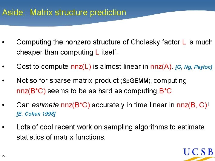
Aside: Matrix structure prediction • Computing the nonzero structure of Cholesky factor L is much cheaper than computing L itself. • Cost to compute nnz(L) is almost linear in nnz(A). [G, Ng, Peyton] • Not so for sparse matrix product (Sp. GEMM); computing nnz(B*C) seems to be as hard as computing B*C. • Can estimate nnz(B*C) accurately in time linear in nnz(B, C)! [E. Cohen 1998] • 27 Lots of cool recent work on sampling algorithms to estimate statistics of matrix functions.

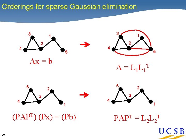
Orderings for sparse Gaussian elimination 3 3 1 2 2 4 5 4 Ax = b 5 5 2 2 3 4 1 (PAPT) (Px) = (Pb) 28 5 A = L 1 L 1 T 3 4 1 1 PAPT = L 2 L 2 T

Nested dissection and graph partitioning [George 1973, many extensions] 29 • Heuristic: Find small vertex separator, put it last, recurse on subgraphs • Theory: Approx optimal separators => approx optimal fill • Practice: Lots of work on heuristics for graph partitioning!

Prehistory: Graph algorithms for sparse matrices Many, many graph algorithms have been used, invented, implemented at large scale for sparse matrix computation: 30 • Symmetric problems: elimination tree, nonzero structure prediction, sparse triangular solve, sparse matrix-matrix multiplication, min-height etree, … • Nonsymmetric problems: sparse triangular solve, bipartite matching (weighted and unweighted), Dulmage-Mendelsohn decomposition / strong components, … • Iterative methods: graph partitioning again, independent set, low-stretch spanning trees, …

History In the year 1992. . . 31

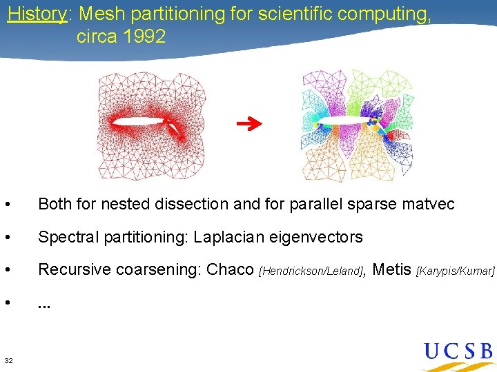
History: Mesh partitioning for scientific computing, circa 1992 • Both for nested dissection and for parallel sparse matvec • Spectral partitioning: Laplacian eigenvectors • Recursive coarsening: Chaco [Hendrickson/Leland], Metis [Karypis/Kumar] • . . . 32

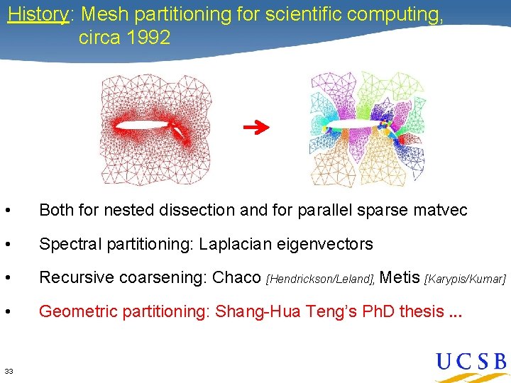
History: Mesh partitioning for scientific computing, circa 1992 • Both for nested dissection and for parallel sparse matvec • Spectral partitioning: Laplacian eigenvectors • Recursive coarsening: Chaco [Hendrickson/Leland], Metis [Karypis/Kumar] • Geometric partitioning: Shang-Hua Teng’s Ph. D thesis. . . 33

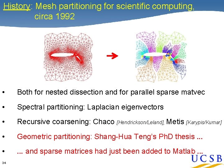
History: Mesh partitioning for scientific computing, circa 1992 • Both for nested dissection and for parallel sparse matvec • Spectral partitioning: Laplacian eigenvectors • Recursive coarsening: Chaco [Hendrickson/Leland], Metis [Karypis/Kumar] • Geometric partitioning: Shang-Hua Teng’s Ph. D thesis. . . • . . . and sparse matrices had just been added to Matlab. . . 34

Geometric partitioning in Matlab [G, Miller, Teng] 5. Projected Back Down 1. Original Mesh Projected D 2. Mesh Points 35 Projected D 3. Stereographic Projection Projected D 4. Conformal Mapping Projected D D 6. Partitioned Mesh

History In the year 2002 (and soon after). . . 36

History In the year 2002 (and soon after). . . (In 2002, JRG shared an office with Jeremy Kepner at MIT. ) 37

First draft of HPCS graph analysis benchmark [circa 2004] 38 • Many tight clusters, loosely interconnected • Input data is edge triples < i, j, a > • Vertices and edges permuted randomly

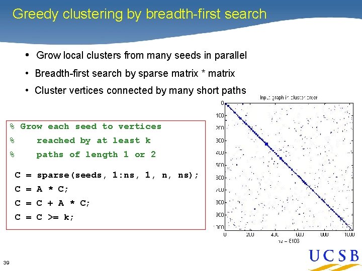
Greedy clustering by breadth-first search • Grow local clusters from many seeds in parallel • Breadth-first search by sparse matrix * matrix • Cluster vertices connected by many short paths % Grow each seed to vertices % reached by at least k % paths of length 1 or 2 C = sparse(seeds, 1: ns, 1, n, ns); C = A * C; C = C + A * C; C = C >= k; 39

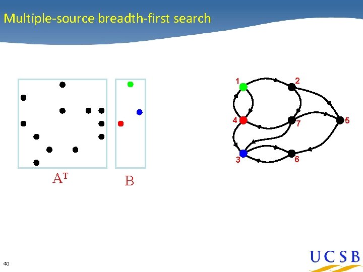
Multiple-source breadth-first search 1 2 4 7 3 AT 40 B 6 5

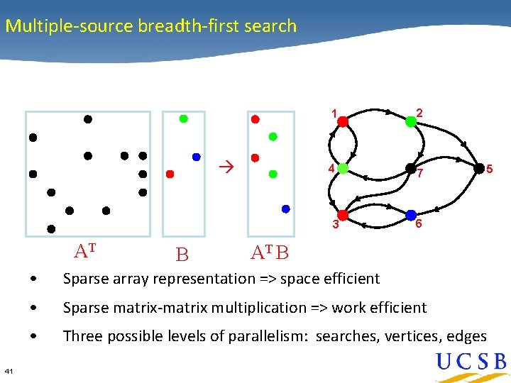
Multiple-source breadth-first search 1 2 4 7 3 AT 41 B 5 6 AT B • Sparse array representation => space efficient • Sparse matrix-matrix multiplication => work efficient • Three possible levels of parallelism: searches, vertices, edges

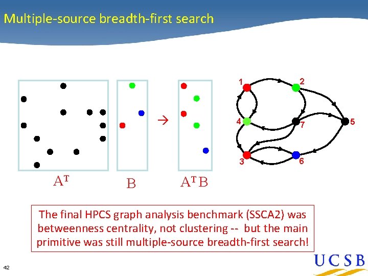
Multiple-source breadth-first search 1 2 4 7 3 AT B 6 AT B The final HPCS graph analysis benchmark (SSCA 2) was betweenness centrality, not clustering -- but the main primitive was still multiple-source breadth-first search! 42 5

History In the year 2010 (and soon after). . . 43

Matrix-based graph processor design at MIT-LL [Song, Kepner, et al. 2010] 44

Combinatorial BLAS [2010] gauss. cs. ucsb. edu/~aydin/Comb. BLAS [Azad, Buluc, G, Lugowski, …] An extensible distributed-memory library offering a small but powerful set of linear algebraic operations specifically targeting graph analytics. • Aimed at graph algorithm designers/programmers who are not expert in mapping algorithms to parallel hardware. • Flexible templated C++ interface. • Scalable performance from laptop to 100, 000 -processor HPC. • Open source software. • Version 1. 6. 2 released April 2018.

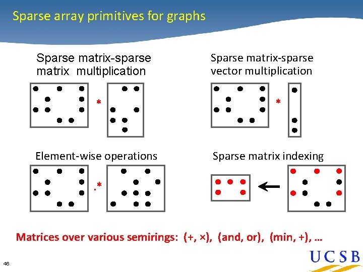
Sparse array primitives for graphs Sparse matrix-sparse matrix multiplication * Element-wise operations Sparse matrix-sparse vector multiplication * Sparse matrix indexing . * Matrices over various semirings: (+, ×), (and, or), (min, +), … 46

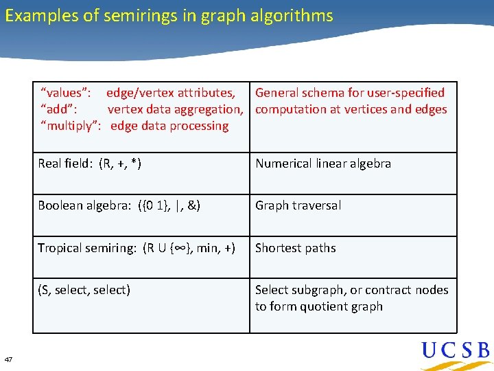
Examples of semirings in graph algorithms “values”: edge/vertex attributes, General schema for user-specified “add”: vertex data aggregation, computation at vertices and edges “multiply”: edge data processing 47 Real field: (R, +, *) Numerical linear algebra Boolean algebra: ({0 1}, |, &) Graph traversal Tropical semiring: (R U {∞}, min, +) Shortest paths (S, select) Select subgraph, or contract nodes to form quotient graph

Graph algorithms in the language of linear algebra • Kepner et al. study [2006]: fundamental graph algorithms including min spanning tree, shortest paths, independent set, max flow, clustering, … • SSCA#2 / centrality [2008] • Basic breadth-first search / Graph 500 [2010] • Combinatorial BLAS [2010] [2011] 48

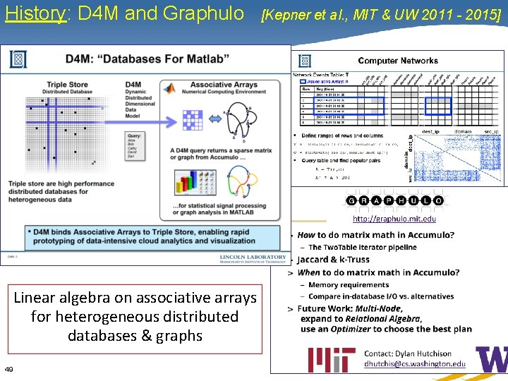
History: D 4 M and Graphulo Linear algebra on associative arrays for heterogeneous distributed databases & graphs 49 [Kepner et al. , MIT & UW 2011 - 2015]

History: Jon Berry challenge problems [2013] • Clustering coefficient (triangle counting) • Connected components (bully algorithm) • Maximum independent set (NP-hard) • Maximal independent set (Luby algorithm) • Single-source shortest paths • Special betweenness (for subgraph isomorphism) 50

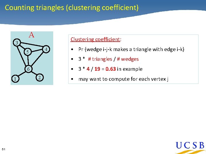
Counting triangles (clustering coefficient) A Clustering coefficient: 3 4 5 • Pr (wedge i-j-k makes a triangle with edge i-k) • 3 * # triangles / # wedges • 3 * 4 / 19 = 0. 63 in example 6 1 51 2 • may want to compute for each vertex j

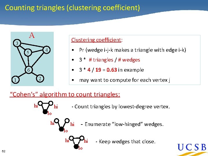
Counting triangles (clustering coefficient) A Clustering coefficient: 3 • Pr (wedge i-j-k makes a triangle with edge i-k) 4 5 • 3 * # triangles / # wedges • 3 * 4 / 19 = 0. 63 in example 6 2 1 • may want to compute for each vertex j “Cohen’s” algorithm to count triangles: hi - Count triangles by lowest-degree vertex. hi lo hi hi - Enumerate “low-hinged” wedges. lo hi 52 hi lo - Keep wedges that close.

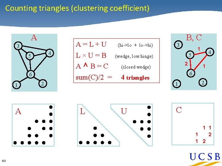
Counting triangles (clustering coefficient) A 3 4 5 6 1 A 2 A=L+U L×U=B A∧ B=C sum(C)/2 = L (hi->lo + lo->hi) 3 B, C 1 2 (closed wedge) 4 triangles U 4 5 (wedge, low hinge) 1 6 1 2 C 1 1 1 2 53

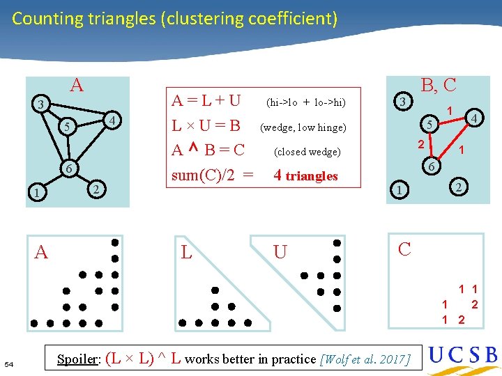
Counting triangles (clustering coefficient) A 3 4 5 6 1 2 A A=L+U L×U=B A∧ B=C sum(C)/2 = L (hi->lo + lo->hi) 3 B, C 1 2 (closed wedge) 4 triangles U 4 5 (wedge, low hinge) 1 6 1 2 C 1 1 1 2 54 Spoiler: (L × L) ^ L works better in practice [Wolf et al. 2017]

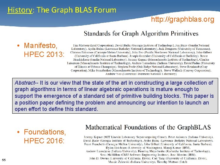
History: The Graph BLAS Forum http: //graphblas. org • Manifesto, HPEC 2013: Abstract-- It is our view that the state of the art in constructing a large collection of graph algorithms in terms of linear algebraic operations is mature enough to support the emergence of a standard set of primitive building blocks. This paper is a position paper defining the problem and announcing our intention to launch an open effort to define this standard. • Foundations, HPEC 2016: 55

The Present In the year 2018. . 56

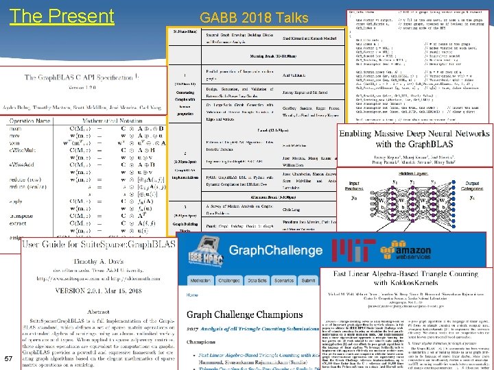
The Present 57 GABB 2018 Talks

The Future In the years 2019 — 58

What do we hope for in the future? • 59 More basic capabilities – Streaming and dynamic-graph algorithms – “Priority queue” algorithms: strong components, top k vertices, etc. – Not materializing intermediate results (eg, incidence matrix methods) – Laplacian paradigm for graph algorithms

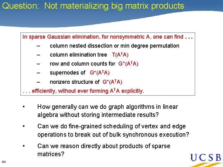
Question: Not materializing big matrix products In sparse Gaussian elimination, for nonsymmetric A, one can find. . . – column nested dissection or min degree permutation – column elimination tree T(ATA) – row and column counts for G+(ATA) – supernodes of G+(ATA) – nonzero structure of G+(ATA) . . . efficiently, without ever forming ATA explicitly. 60 • How generally can we do graph algorithms in linear algebra without storing intermediate results? • Can we do fine-grained scheduling of vertex and edge operations to break out of bulk synchronous execution? • Can we reason directly about products of sparse matrices?

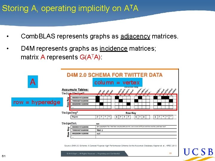
Storing A, operating implicitly on ATA • Comb. BLAS represents graphs as adjacency matrices. • D 4 M represents graphs as incidence matrices; matrix A represents G(ATA): A row = hyperedge 61 column = vertex

Storing A, operating implicitly on ATA • • 62 Many other cases: – Optimization: KKT systems, interior point methods. – Automatic differentiation: distance-2 coloring. – Linear equations: QR factorization, structure prediction for LU factorization with partial pivoting. Question: What can you do fast on G(ATA) just from G(A)?

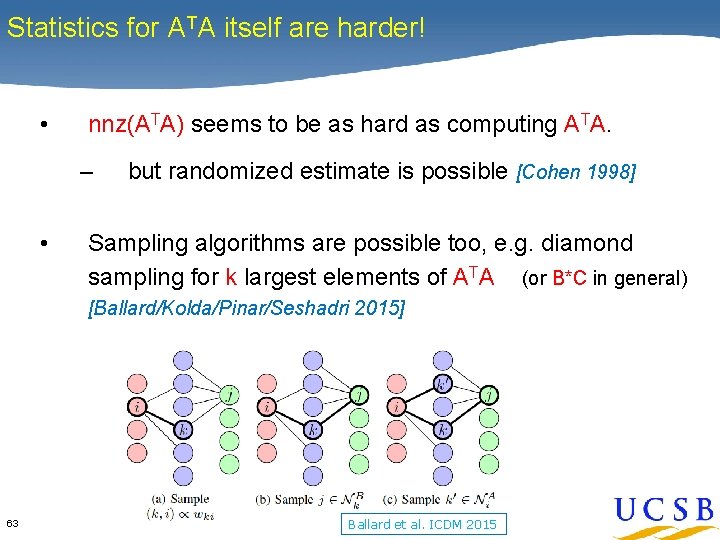
Statistics for ATA itself are harder! • nnz(ATA) seems to be as hard as computing ATA. – • but randomized estimate is possible [Cohen 1998] Sampling algorithms are possible too, e. g. diamond sampling for k largest elements of ATA (or B*C in general) [Ballard/Kolda/Pinar/Seshadri 2015] 63 Ballard et al. ICDM 2015

What do we hope for in the future? • 64 More basic capabilities – Streaming and dynamic algorithms – “Priority queue” algorithms: strong components, top k vertices, etc. – Not materializing intermediate results (eg, incidence matrix methods) – Laplacian paradigm for graph algorithms

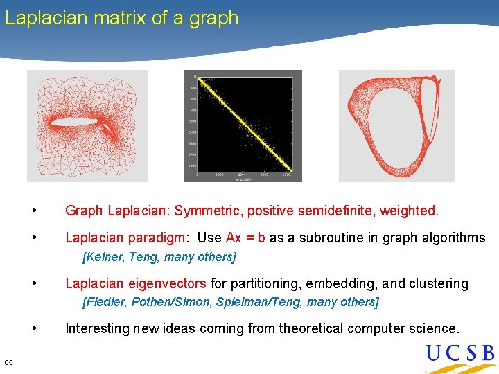
Laplacian matrix of a graph • Graph Laplacian: Symmetric, positive semidefinite, weighted. • Laplacian paradigm: Use Ax = b as a subroutine in graph algorithms [Kelner, Teng, many others] • Laplacian eigenvectors for partitioning, embedding, and clustering [Fiedler, Pothen/Simon, Spielman/Teng, many others] • 65 Interesting new ideas coming from theoretical computer science.

What do we hope for in the future? • 66 More basic capabilities – Streaming and dynamic algorithms – “Priority queue” algorithms: strong components, top k vertices, etc. – Not materializing intermediate results (eg, incidence matrix methods) – Laplacian paradigm for graph algorithms

What do we hope for in the future? • • 67 More basic capabilities – Streaming and dynamic algorithms – “Priority queue” algorithms: strong components, top k vertices, etc. – Not materializing intermediate results (eg, incidence matrix methods) – Laplacian paradigm for graph algorithms More directions – Integration with numerical matrix libraries – Statistical perspective: random objects, stochastic graphs, etc. – Deep neural networks (more) – Signal processing on graphs

What do we hope for in the future? • • • 68 More basic capabilities – Streaming and dynamic algorithms – “Priority queue” algorithms: strong components, top k vertices, etc. – Not materializing intermediate results (eg, incidence matrix methods) – Laplacian paradigm for graph algorithms More directions – Integration with numerical matrix libraries – Statistical perspective: random objects, stochastic graphs, etc. – Deep neural networks (more) – Signal processing on graphs More uptake – By hardware vendors – By software vendors

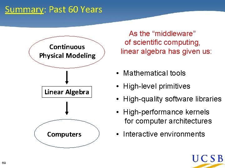
Summary: Past 60 Years Continuous Physical Modeling As the “middleware” of scientific computing, linear algebra has given us: • Mathematical tools Linear Algebra • High-level primitives • High-quality software libraries • High-performance kernels for computer architectures Computers 69 • Interactive environments

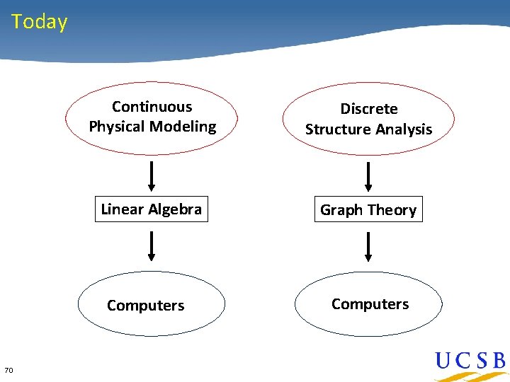
Today Continuous Physical Modeling Discrete Structure Analysis Linear Algebra Graph Theory Computers 70 Computers

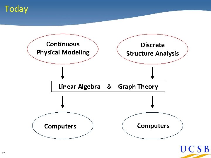
Today Continuous Physical Modeling Discrete Structure Analysis Linear Algebra & Graph Theory Computers 71 Computers

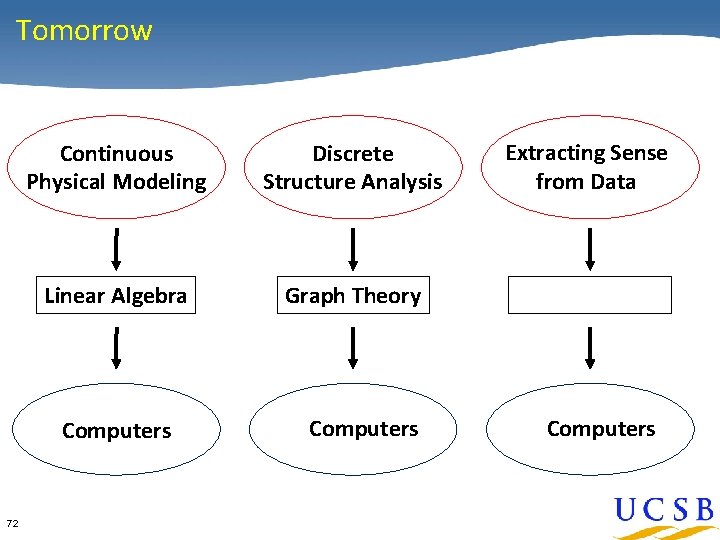
Tomorrow Continuous Physical Modeling Discrete Structure Analysis Extracting Sense from Data Linear Algebra Graph Theory Mae Learning? Computers 72 Computers

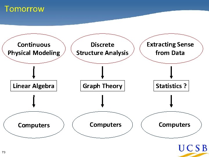
Tomorrow Continuous Physical Modeling Discrete Structure Analysis Extracting Sense from Data Linear Algebra Graph Theory Statistics ? Computers 73 Computers

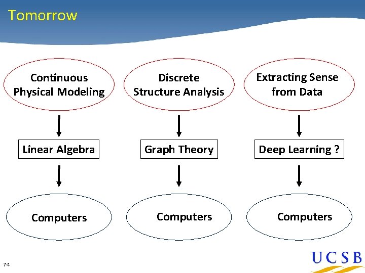
Tomorrow Continuous Physical Modeling Discrete Structure Analysis Extracting Sense from Data Linear Algebra Graph Theory Deep Learning ? Computers 74 Computers

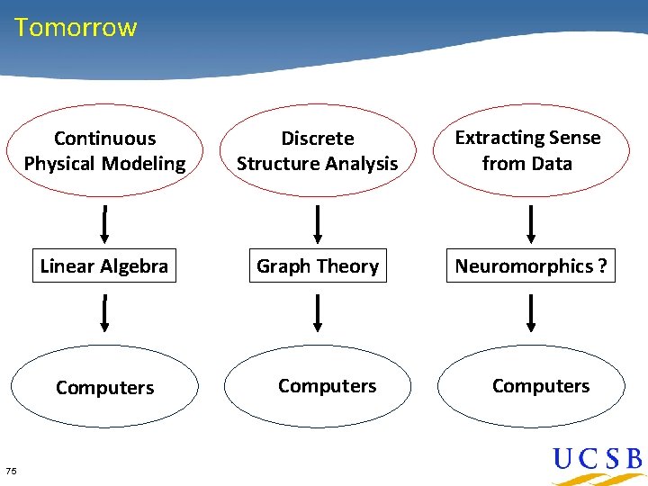
Tomorrow Continuous Physical Modeling Discrete Structure Analysis Extracting Sense from Data Linear Algebra Graph Theory Neuromorphics ? Computers 75 Computers

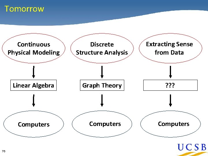
Tomorrow Continuous Physical Modeling Discrete Structure Analysis Extracting Sense from Data Linear Algebra Graph Theory xxaine? ? ? earngx Computers 76 Computers

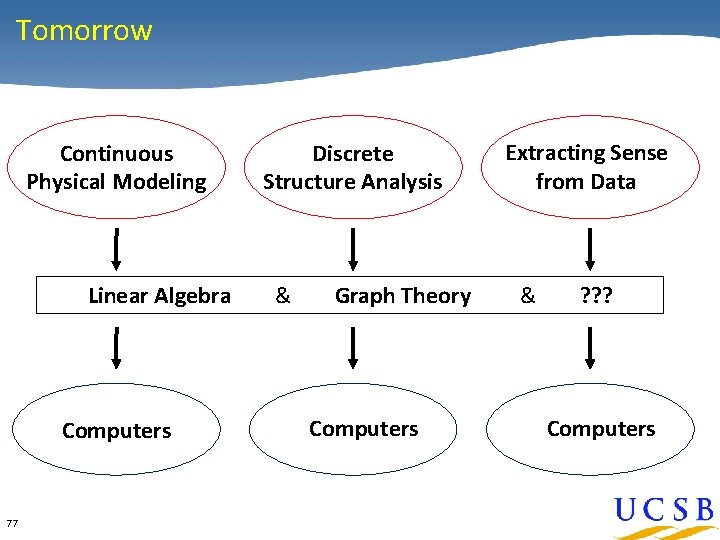
Tomorrow Continuous Physical Modeling Linear Algebra Computers 77 Discrete Structure Analysis & Graph Theory Computers Extracting Sense from Data & ? ? ? Computers

Thanks … Ariful Azad, David Bader, Jon Berry, Eric Boman, Aydin Buluc, Ben Chang, John Conroy, Tim Davis, Kevin Deweese, Erika Duriakova, Assefaw Gebremedhin, Shoaib Kamil, Jeremy Kepner, Tammy Kolda, Tristan Konolige, Manoj Kumar, Adam Lugowski, Tim Mattson, Scott Mc. Millan, Henning Meyerhenke, Jose Moreira, Esmond Ng, Lenny Oliker, Weimin Ouyang, Ali Pinar, Alex Pothen, Carey Priebe, Steve Reinhardt, Lijie Ren, Eric Robinson, Viral Shah, Veronika Strnadova-Neeley, Blair Sullivan, Shang-Hua Teng, Yun Teng, Sam Williams 78 … and Intel, Microsoft, NSF, DOE Office of Science