Graph Algorithms Counting Triangles Transitive Closure Jeffrey D

Graph Algorithms Counting Triangles Transitive Closure Jeffrey D. Ullman Stanford University/Infolab

Counting Triangles Bounds on Numbers of Triangles Heavy Hitters An Optimal Algorithm

Counting Triangles �Why Care? 1. Density of triangles measures maturity of a community. § As communities age, their members tend to connect. 2. The algorithm is actually an example of a recent and powerful theory of optimal join computation. 3

Data Structures Needed �We need to represent a graph by data structures that let us do two things efficiently: 1. Given nodes u and v, determine whethere exists an edge between them in O(1) time. 2. Find the edges out of a node in time proportional to the number of those edges. � Question for thought: What data structures would you recommend? 4

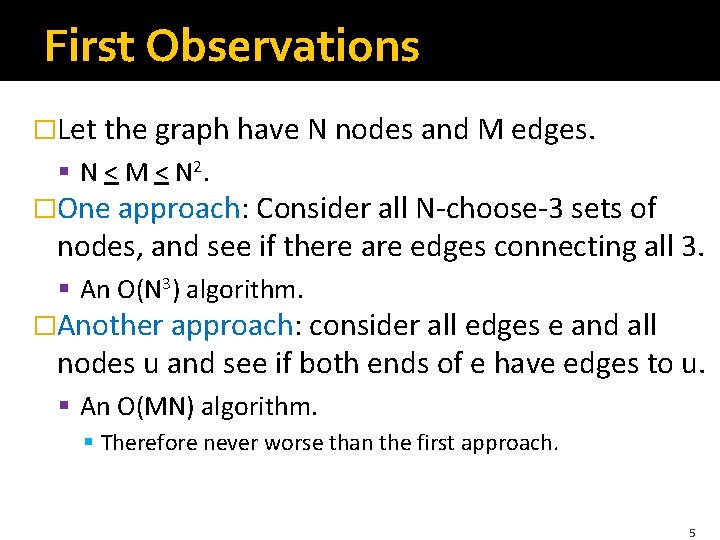
First Observations �Let the graph have N nodes and M edges. § N < M < N 2. �One approach: Consider all N-choose-3 sets of nodes, and see if there are edges connecting all 3. § An O(N 3) algorithm. �Another approach: consider all edges e and all nodes u and see if both ends of e have edges to u. § An O(MN) algorithm. § Therefore never worse than the first approach. 5

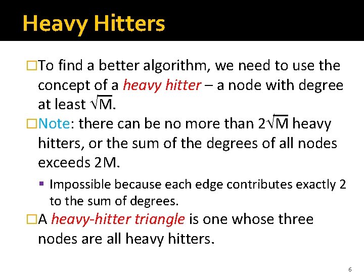
Heavy Hitters �To find a better algorithm, we need to use the concept of a heavy hitter – a node with degree at least M. �Note: there can be no more than 2 M heavy hitters, or the sum of the degrees of all nodes exceeds 2 M. § Impossible because each edge contributes exactly 2 to the sum of degrees. �A heavy-hitter triangle is one whose three nodes are all heavy hitters. 6

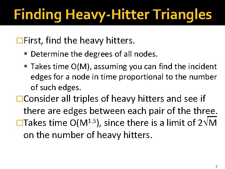
Finding Heavy-Hitter Triangles �First, find the heavy hitters. § Determine the degrees of all nodes. § Takes time O(M), assuming you can find the incident edges for a node in time proportional to the number of such edges. �Consider all triples of heavy hitters and see if there are edges between each pair of the three. �Takes time O(M 1. 5), since there is a limit of 2 M on the number of heavy hitters. 7

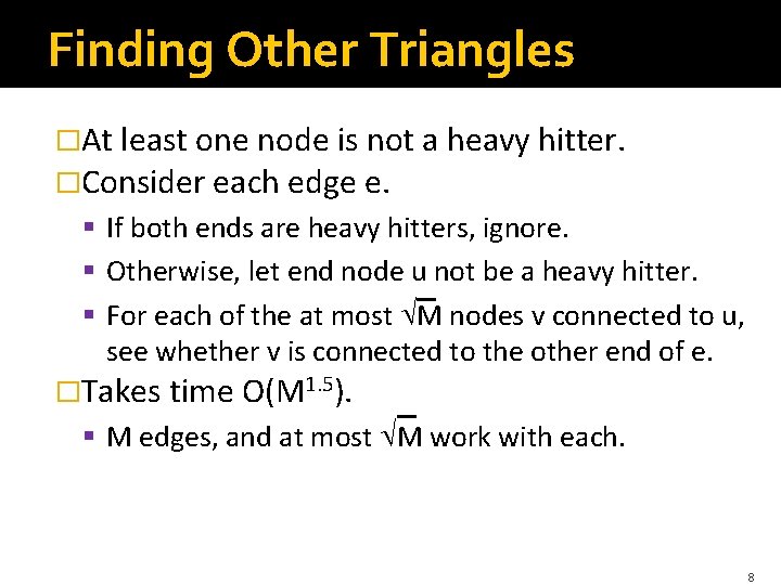
Finding Other Triangles �At least one node is not a heavy hitter. �Consider each edge e. § If both ends are heavy hitters, ignore. § Otherwise, let end node u not be a heavy hitter. § For each of the at most M nodes v connected to u, see whether v is connected to the other end of e. �Takes time O(M 1. 5). § M edges, and at most M work with each. 8

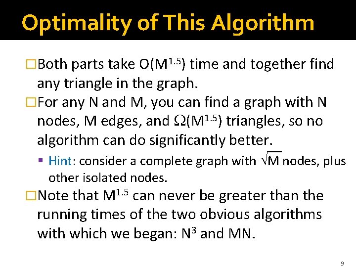
Optimality of This Algorithm �Both parts take O(M 1. 5) time and together find any triangle in the graph. �For any N and M, you can find a graph with N nodes, M edges, and (M 1. 5) triangles, so no algorithm can do significantly better. § Hint: consider a complete graph with M nodes, plus other isolated nodes. �Note that M 1. 5 can never be greater than the running times of the two obvious algorithms with which we began: N 3 and MN. 9

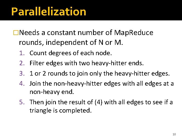
Parallelization �Needs a constant number of Map. Reduce rounds, independent of N or M. 1. 2. 3. 4. Count degrees of each node. Filter edges with two heavy-hitter ends. 1 or 2 rounds to join only the heavy-hitter edges. Join the non-heavy-hitter edges with all edges at a non-heavy end. 5. Then join the result of (4) with all edges to see if a triangle is completed. 10

Transitive Closure Classical Approaches Arc + Path => Path “Smart” Transitive Closure Strongly Connected Components

Issues Regarding Parallelism �Different algorithms for the same problem can be parallelized to different degrees. �The same activity can (sometimes) be performed for each node in parallel. �A relational join or similar step can be performed in one round of Map. Reduce. �Parameters: N = # nodes, M = # edges, D = diameter. 12

The Setting �A directed graph of N nodes and M arcs. �Arcs are represented by a relation Arc(u, v) meaning there is an arc from node u to node v. �Goal is to compute the transitive closure of Arc, which is the relation Path(u, v), meaning that there is a path of length 1 or more from u to v. �Bad news: TC takes (serial) time O(NM) in the worst case. �Good news: But you can parallelize it heavily. 13

Why Transitive Closure? �Important in its own right. § Finding structure of the Web, e. g. , strongly connected “central” region. § Finding connections: “was money ever transferred, directly or indirectly, from the West-Side Mob to the Stanford Chess Club? ” § Ancestry: “is Jeff Ullman a descendant of Genghis Khan? ” �Every linear recursion (only one recursive call) can be expressed as a transitive closure plus nonrecursive stuff to translate to and from TC. 14

Classical Methods for TC Warshall’s Algorithm Depth-First Search Breadth-First Search

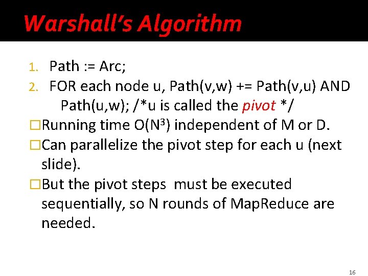
Warshall’s Algorithm Path : = Arc; FOR each node u, Path(v, w) += Path(v, u) AND Path(u, w); /*u is called the pivot */ �Running time O(N 3) independent of M or D. �Can parallelize the pivot step for each u (next slide). �But the pivot steps must be executed sequentially, so N rounds of Map. Reduce are needed. 1. 2. 16

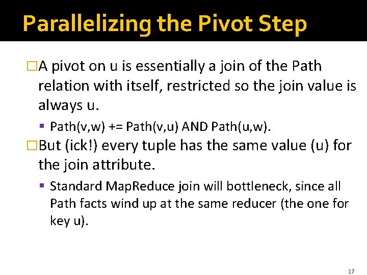
Parallelizing the Pivot Step �A pivot on u is essentially a join of the Path relation with itself, restricted so the join value is always u. § Path(v, w) += Path(v, u) AND Path(u, w). �But (ick!) every tuple has the same value (u) for the join attribute. § Standard Map. Reduce join will bottleneck, since all Path facts wind up at the same reducer (the one for key u). 17

Skew Joins �This problem, where one or more values of the join attribute are “heavy hitters” is called skew. �It limits the amount of parallelism, unless you do something clever. �But there is a cost: in Map. Reduce terms, you communicate each Path fact from its mapper to many reducers. § As communication is often the bottleneck, you have to be clever how you parallelize when there is a heavy hitter. 18

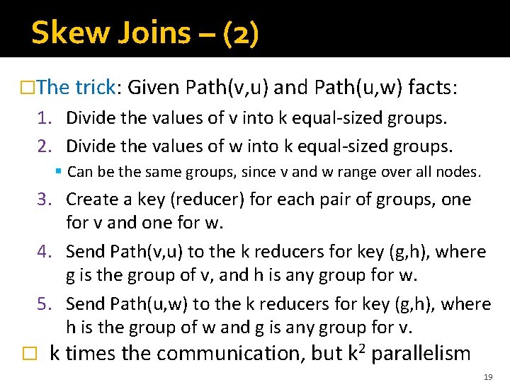
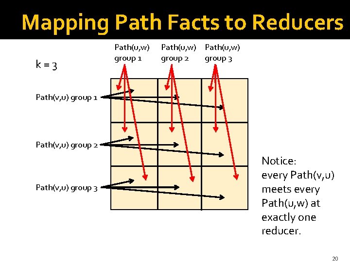
Skew Joins – (2) �The trick: Given Path(v, u) and Path(u, w) facts: 1. Divide the values of v into k equal-sized groups. 2. Divide the values of w into k equal-sized groups. § Can be the same groups, since v and w range over all nodes. 3. Create a key (reducer) for each pair of groups, one for v and one for w. 4. Send Path(v, u) to the k reducers for key (g, h), where g is the group of v, and h is any group for w. 5. Send Path(u, w) to the k reducers for key (g, h), where h is the group of w and g is any group for v. � k times the communication, but k 2 parallelism 19

Mapping Path Facts to Reducers k=3 Path(u, w) group 1 Path(u, w) group 2 group 3 Path(v, u) group 1 Path(v, u) group 2 Path(v, u) group 3 Notice: every Path(v, u) meets every Path(u, w) at exactly one reducer. 20

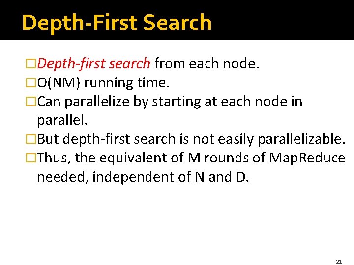
Depth-First Search �Depth-first search from each node. �O(NM) running time. �Can parallelize by starting at each node in parallel. �But depth-first search is not easily parallelizable. �Thus, the equivalent of M rounds of Map. Reduce needed, independent of N and D. 21

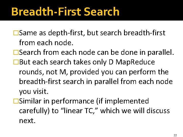
Breadth-First Search �Same as depth-first, but search breadth-first from each node. �Search from each node can be done in parallel. �But each search takes only D Map. Reduce rounds, not M, provided you can perform the breadth-first search in parallel from each node you visit. �Similar in performance (if implemented carefully) to “linear TC, ” which we will discuss next. 22

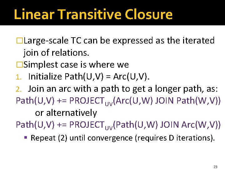
Linear Transitive Closure �Large-scale TC can be expressed as the iterated join of relations. �Simplest case is where we 1. Initialize Path(U, V) = Arc(U, V). 2. Join an arc with a path to get a longer path, as: Path(U, V) += PROJECTUV(Arc(U, W) JOIN Path(W, V)) or alternatively Path(U, V) += PROJECTUV(Path(U, W) JOIN Arc(W, V)) § Repeat (2) until convergence (requires D iterations). 23

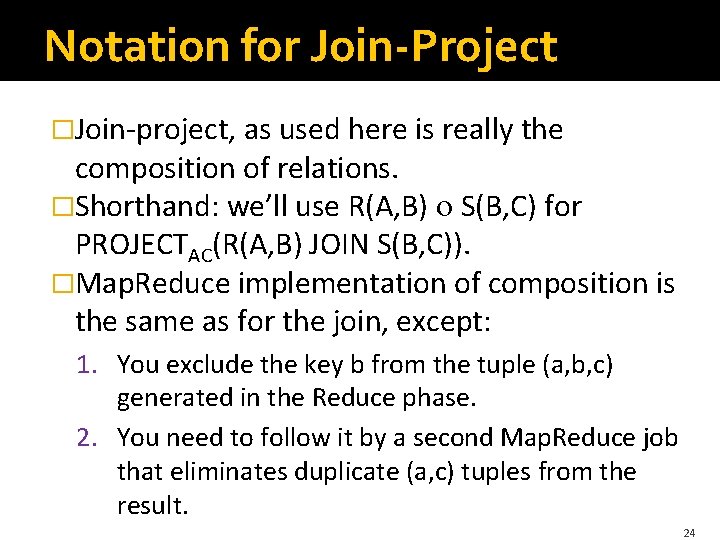
Notation for Join-Project �Join-project, as used here is really the composition of relations. �Shorthand: we’ll use R(A, B) S(B, C) for PROJECTAC(R(A, B) JOIN S(B, C)). �Map. Reduce implementation of composition is the same as for the join, except: 1. You exclude the key b from the tuple (a, b, c) generated in the Reduce phase. 2. You need to follow it by a second Map. Reduce job that eliminates duplicate (a, c) tuples from the result. 24

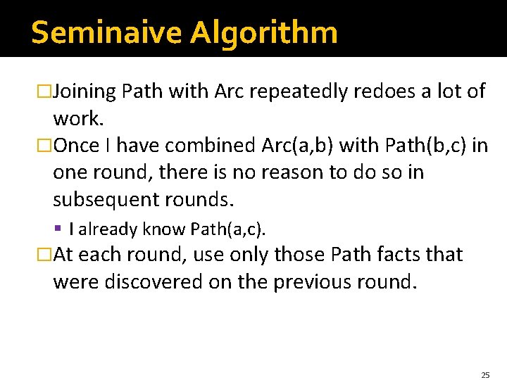
Seminaive Algorithm �Joining Path with Arc repeatedly redoes a lot of work. �Once I have combined Arc(a, b) with Path(b, c) in one round, there is no reason to do so in subsequent rounds. § I already know Path(a, c). �At each round, use only those Path facts that were discovered on the previous round. 25

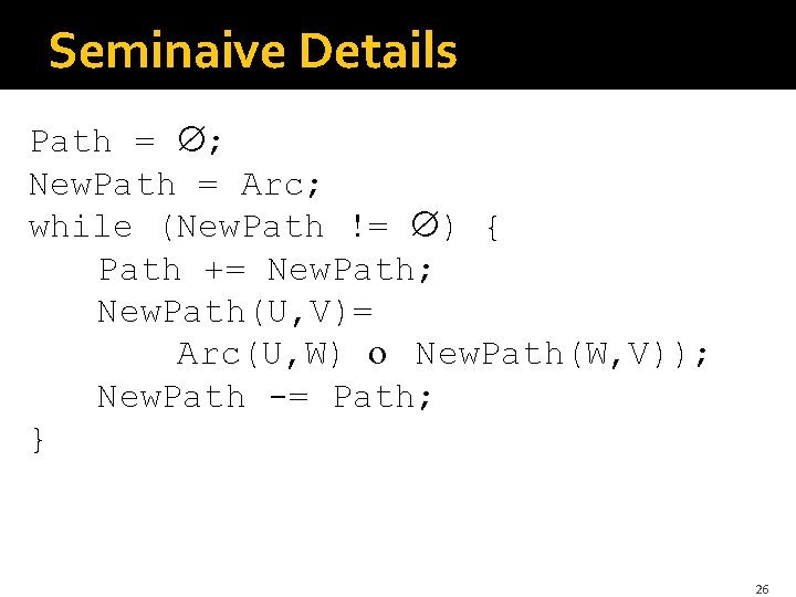
Seminaive Details Path = ; New. Path = Arc; while (New. Path != ) { Path += New. Path; New. Path(U, V)= Arc(U, W) New. Path(W, V)); New. Path -= Path; } 26

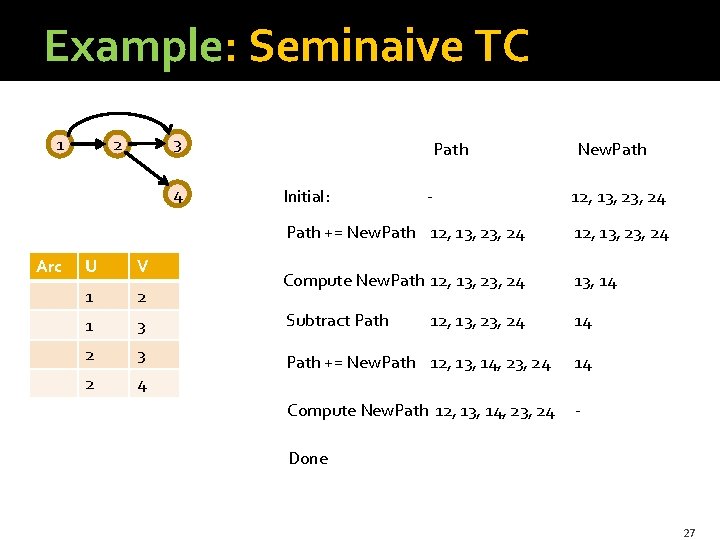
Example: Seminaive TC 1 3 2 4 Arc Path Initial: - New. Path 12, 13, 24 Path += New. Path 12, 13, 23, 24 Compute New. Path 12, 13, 24 13, 14 14 U V 1 2 1 3 Subtract Path 2 3 2 4 Path += New. Path 12, 13, 14, 23, 24 14 Compute New. Path 12, 13, 14, 23, 24 - 12, 13, 24 Done 27

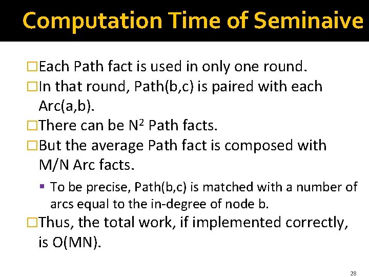
Computation Time of Seminaive �Each Path fact is used in only one round. �In that round, Path(b, c) is paired with each Arc(a, b). �There can be N 2 Path facts. �But the average Path fact is composed with M/N Arc facts. § To be precise, Path(b, c) is matched with a number of arcs equal to the in-degree of node b. �Thus, the total work, if implemented correctly, is O(MN). 28

How Many Rounds? �Each round of seminaive TC requires two Map. Reduce jobs. § One to join, the other to eliminate duplicates. �Number of rounds needed equals the diameter. § More parallelizable than classical methods (or equivalent to breadth-first search) when D is small. 29

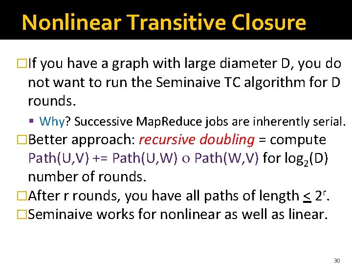
Nonlinear Transitive Closure �If you have a graph with large diameter D, you do not want to run the Seminaive TC algorithm for D rounds. § Why? Successive Map. Reduce jobs are inherently serial. �Better approach: recursive doubling = compute Path(U, V) += Path(U, W) Path(W, V) for log 2(D) number of rounds. �After r rounds, you have all paths of length < 2 r. �Seminaive works for nonlinear as well as linear. 30

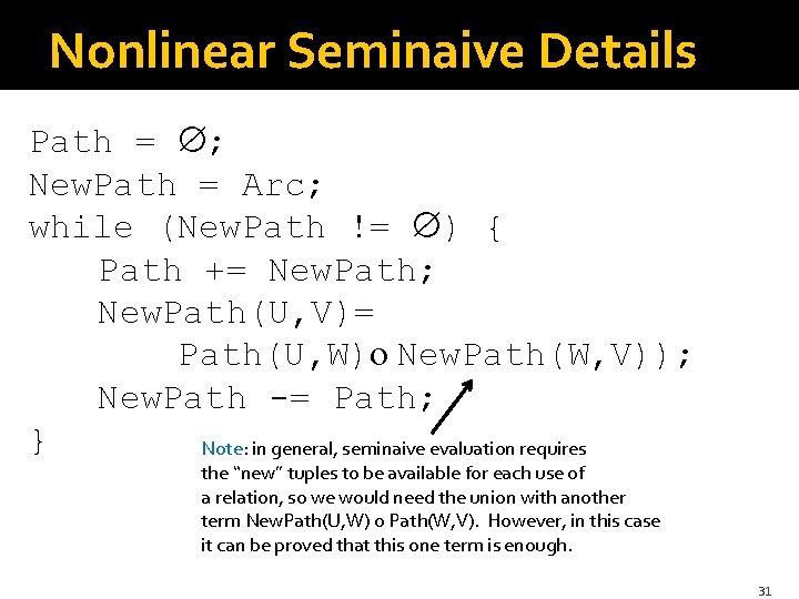
Nonlinear Seminaive Details Path = ; New. Path = Arc; while (New. Path != ) { Path += New. Path; New. Path(U, V)= Path(U, W) New. Path(W, V)); New. Path -= Path; } Note: in general, seminaive evaluation requires the “new” tuples to be available for each use of a relation, so we would need the union with another term New. Path(U, W) o Path(W, V). However, in this case it can be proved that this one term is enough. 31

Computation Time of Nonlinear + Seminaive �Each Path fact is in New. Path only once. �There can be N 2 Path facts. �When (a, b) is in New. Path, it can be joined with N other Path facts. § Those of the form Path(x, a). �Thus, total computation is O(N 3). § Looks worse than the O(MN) we derived for linear TC. 32

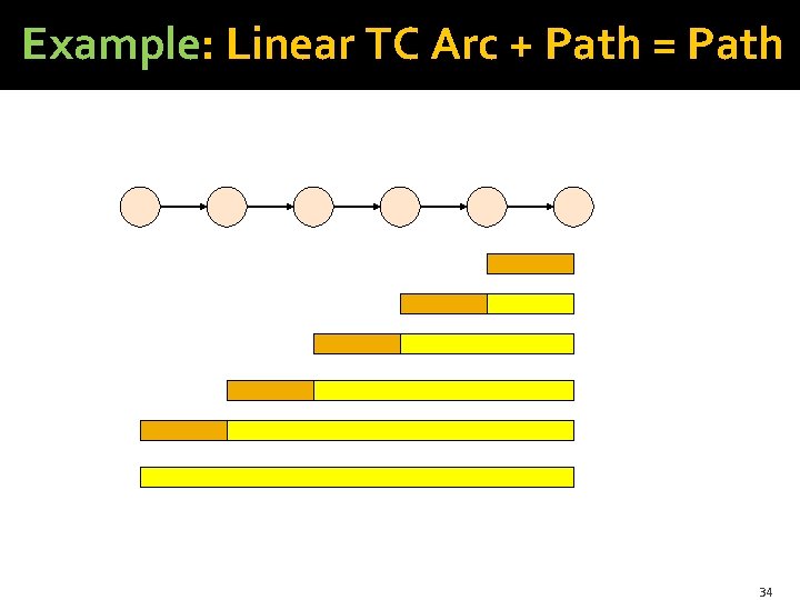
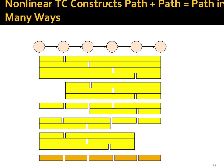
A Problem With Nonlinear TC �Good news: You generate the same Path facts as for linear TC, but in fewer rounds, often a lot fewer. �Bad news: you generate the same fact in many different ways, compared with linear. �Neither method can avoid the fact that if there are many different paths from u to v, you will discover each of those paths, even though one would be enough. �But nonlinear discovers the same exact path many times. 33

Example: Linear TC Arc + Path = Path 34

Nonlinear TC Constructs Path + Path = Path in Many Ways 35

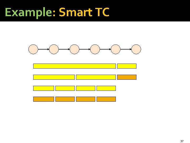
Smart TC � (Valduriez-Boral, Ioannides) Construct a path from two paths: 1. The first has a length that is a power of 2. 2. The second is no longer than the first. 36

Example: Smart TC 37

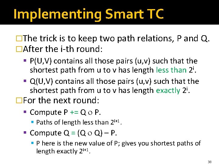
Implementing Smart TC �The trick is to keep two path relations, P and Q. �After the i-th round: § P(U, V) contains all those pairs (u, v) such that the shortest path from u to v has length less than 2 i. § Q(U, V) contains all those pairs (u, v) such that the shortest path from u to v has length exactly 2 i. �For the next round: § Compute P += Q P. § Paths of length less than 2 i+1. § Compute Q = (Q Q) – P. § P here is the new value of P; gives you shortest paths of length exactly 2 i+1. 38

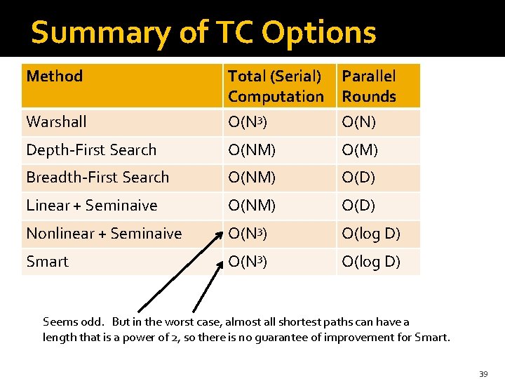
Summary of TC Options Method Warshall Total (Serial) Computation O(N 3) Parallel Rounds O(N) Depth-First Search O(NM) O(M) Breadth-First Search O(NM) O(D) Linear + Seminaive O(NM) O(D) Nonlinear + Seminaive O(N 3) O(log D) Smart O(N 3) O(log D) Seems odd. But in the worst case, almost all shortest paths can have a length that is a power of 2, so there is no guarantee of improvement for Smart. 39

Graphs With Large Cycles �In a sense, acyclic graphs are the hardest TC cases. �If there are large strongly connected components (SCC’s) = sets of nodes with a path from any member of the set to any other, you can simplify TC. �Example: The Web has a large SCC and other acyclic structures (see Sect. 5. 1. 3). § The big SCC and other SCC’s made it much easier to discover the structure of the Web. 40

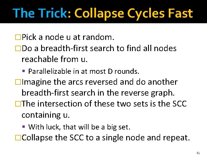
The Trick: Collapse Cycles Fast �Pick a node u at random. �Do a breadth-first search to find all nodes reachable from u. § Parallelizable in at most D rounds. �Imagine the arcs reversed and do another breadth-first search in the reverse graph. �The intersection of these two sets is the SCC containing u. § With luck, that will be a big set. �Collapse the SCC to a single node and repeat. 41

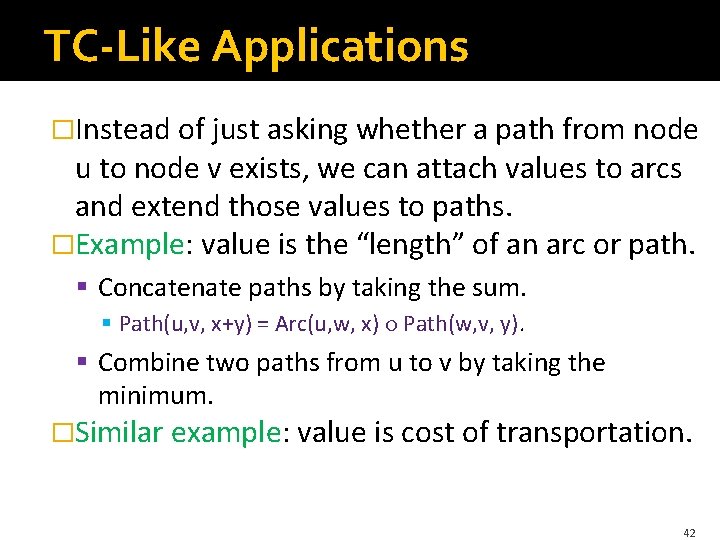
TC-Like Applications �Instead of just asking whether a path from node u to node v exists, we can attach values to arcs and extend those values to paths. �Example: value is the “length” of an arc or path. § Concatenate paths by taking the sum. § Path(u, v, x+y) = Arc(u, w, x) Path(w, v, y). § Combine two paths from u to v by taking the minimum. �Similar example: value is cost of transportation. 42