Graph Algorithms Comp 550 Graph G V E

Graph Algorithms Comp 550

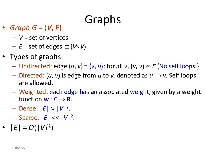
• Graph G = (V, E) Graphs – V = set of vertices – E = set of edges (V V) • Types of graphs – Undirected: edge (u, v) = (v, u); for all v, (v, v) E (No self loops. ) – Directed: (u, v) is edge from u to v, denoted as u v. Self loops are allowed. – Weighted: each edge has an associated weight, given by a weight function w : E R. – Dense: |E| |V|2. – Sparse: |E| << |V|2. • |E| = O(|V|2) Comp 550

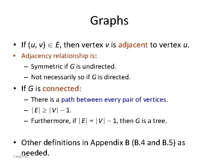
Graphs • If (u, v) E, then vertex v is adjacent to vertex u. • Adjacency relationship is: – Symmetric if G is undirected. – Not necessarily so if G is directed. • If G is connected: – There is a path between every pair of vertices. – |E| |V| – 1. – Furthermore, if |E| = |V| – 1, then G is a tree. • Other definitions in Appendix B (B. 4 and B. 5) as needed. Comp 550

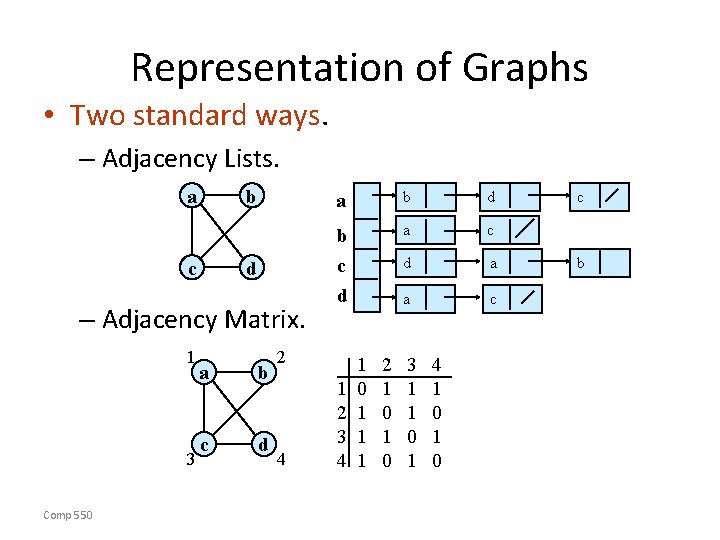
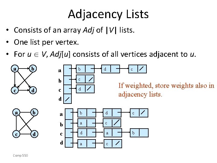
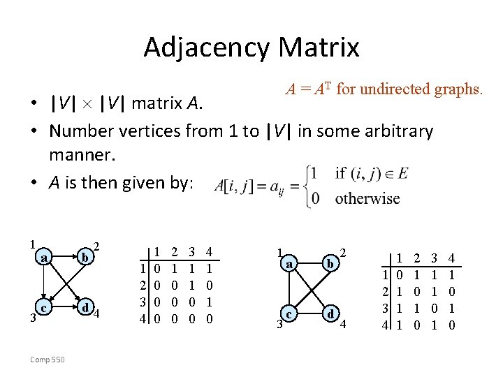
Representation of Graphs • Two standard ways. – Adjacency Lists. a c b a b d a c d b c d d a a c – Adjacency Matrix. 1 3 Comp 550 a b c d 2 4 1 2 3 4 1 0 1 1 1 2 1 0 3 1 1 0 1 4 1 0 c b

Adjacency Lists • Consists of an array Adj of |V| lists. • One list per vertex. • For u V, Adj[u] consists of all vertices adjacent to u. a b c c d b c d a b d a c d b c d d a a c c Comp 550 d c If weighted, store weights also in adjacency lists. d c b

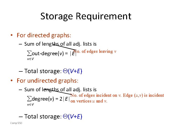
Storage Requirement • For directed graphs: – Sum of lengths of all adj. lists is No. of edges leaving v out-degree(v) = |E| v V – Total storage: (V+E) • For undirected graphs: – Sum of lengths of all adj. lists is No. of edges incident on v. Edge (u, v) is incident degree(v) = 2|E|on vertices u and v. v V – Total storage: (V+E) Comp 550

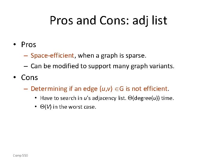
Pros and Cons: adj list • Pros – Space-efficient, when a graph is sparse. – Can be modified to support many graph variants. • Cons – Determining if an edge (u, v) G is not efficient. • Have to search in u’s adjacency list. (degree(u)) time. • (V) in the worst case. Comp 550

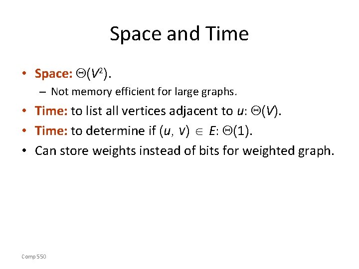
Adjacency Matrix A = AT for undirected graphs. • |V| matrix A. • Number vertices from 1 to |V| in some arbitrary manner. • A is then given by: 1 3 a c Comp 550 b 2 d 4 1 2 3 4 1 0 0 2 1 0 0 0 3 1 1 0 0 4 1 0 1 3 a b c d 2 4 1 2 3 4 1 0 1 1 1 2 1 0 3 1 1 0 1 4 1 0

Space and Time • Space: (V 2). – Not memory efficient for large graphs. • Time: to list all vertices adjacent to u: (V). • Time: to determine if (u, v) E: (1). • Can store weights instead of bits for weighted graph. Comp 550

Graph-searching Algorithms • Searching a graph: – Systematically follow the edges of a graph to visit the vertices of the graph. • Used to discover the structure of a graph. • Standard graph-searching algorithms. – Breadth-first Search (BFS). – Depth-first Search (DFS). Comp 550

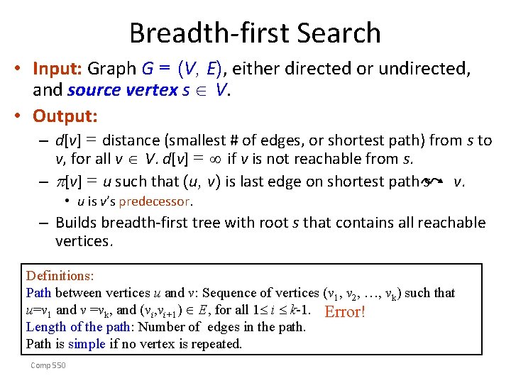
Breadth-first Search • Input: Graph G = (V, E), either directed or undirected, and source vertex s V. • Output: – d[v] = distance (smallest # of edges, or shortest path) from s to v, for all v V. d[v] = if v is not reachable from s. – [v] = u such that (u, v) is last edge on shortest path s v. • u is v’s predecessor. – Builds breadth-first tree with root s that contains all reachable vertices. Definitions: Path between vertices u and v: Sequence of vertices (v 1, v 2, …, vk) such that u=v 1 and v =vk, and (vi, vi+1) E, for all 1 i k-1. Error! Length of the path: Number of edges in the path. Path is simple if no vertex is repeated. Comp 550

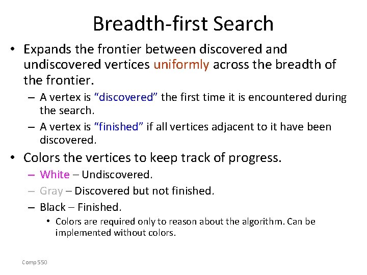
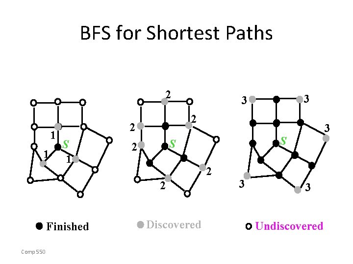
Breadth-first Search • Expands the frontier between discovered and undiscovered vertices uniformly across the breadth of the frontier. – A vertex is “discovered” the first time it is encountered during the search. – A vertex is “finished” if all vertices adjacent to it have been discovered. • Colors the vertices to keep track of progress. – White – Undiscovered. – Gray – Discovered but not finished. – Black – Finished. • Colors are required only to reason about the algorithm. Can be implemented without colors. Comp 550

BFS for Shortest Paths 2 1 1 2 2 S 1 Comp 550 3 S S 2 2 2 Finished 3 3 Discovered 3 3 Undiscovered

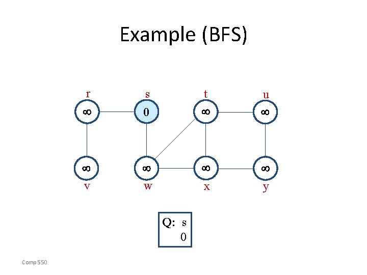
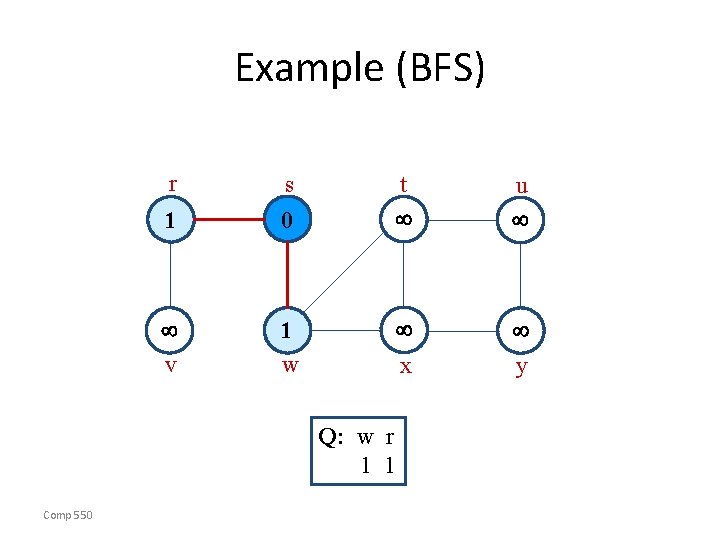
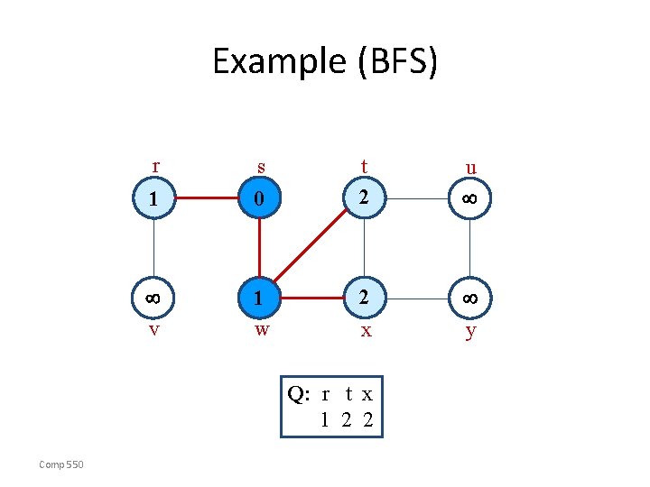
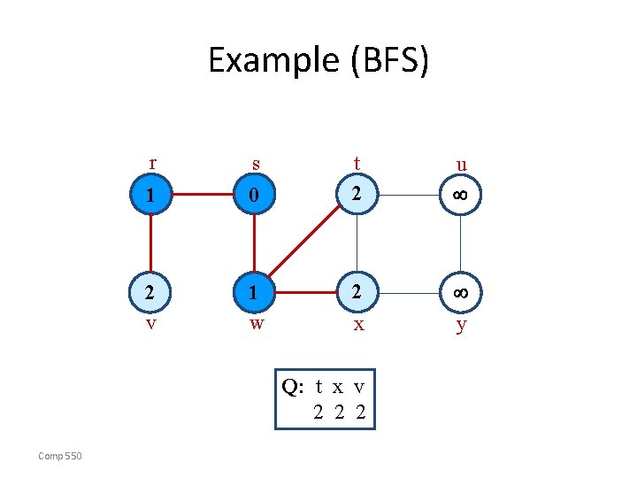
BFS(G, s) 1. for each vertex u in V[G] – {s} 2 do color[u] white 3 d[u] 4 [u] nil 5 color[s] gray 6 d[s] 0 7 [s] nil 8 Q 9 enqueue(Q, s) 10 while Q 11 do u dequeue(Q) 12 for each v in Adj[u] 13 do if color[v] = white 14 then color[v] gray 15 d[v] d[u] + 1 16 [v] u 17 enqueue(Q, v) 18 color[u] black Comp 550 white: undiscovered gray: discovered black: finished Q: a queue of discovered vertices color[v]: color of v d[v]: distance from s to v [u]: predecessor of v Example: animation.

Example (BFS) r 0 v w s u y x Q: s 0 Comp 550 t

Example (BFS) r s 1 0 v 1 w t u y x Q: w r 1 1 Comp 550

Example (BFS) r s 1 0 v 1 w t 2 u 2 y x Q: r t x 1 2 2 Comp 550

Example (BFS) r s 1 0 2 v 1 w t 2 u 2 y x Q: t x v 2 2 2 Comp 550

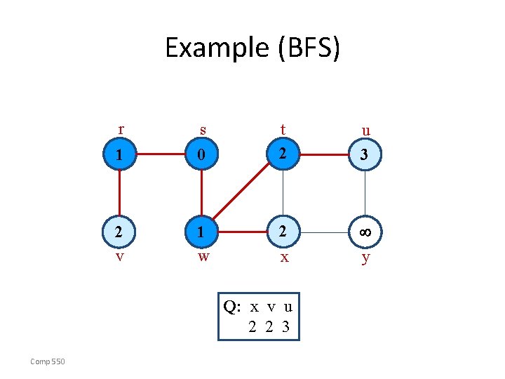
Example (BFS) r s 1 0 2 v 1 w t 2 u 3 2 y x Q: x v u 2 2 3 Comp 550

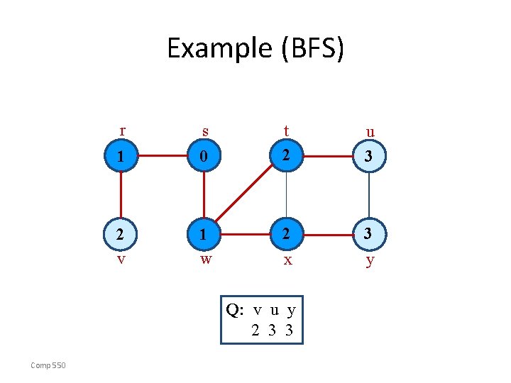
Example (BFS) r s 1 0 2 v 1 w t 2 u 3 2 3 y x Q: v u y 2 3 3 Comp 550

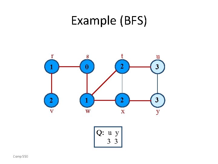
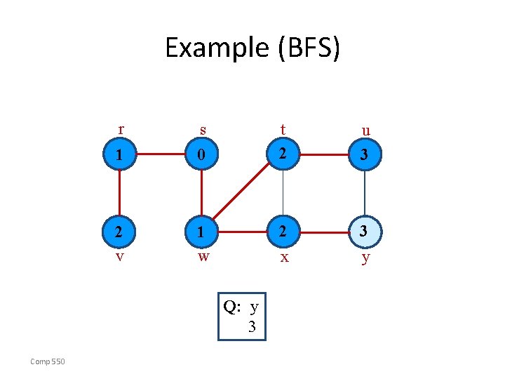
Example (BFS) r s 1 0 2 v 1 w u 3 2 3 y x Q: u y 3 3 Comp 550 t 2

Example (BFS) r s 1 0 2 v 1 w u 3 2 3 y x Q: y 3 Comp 550 t 2

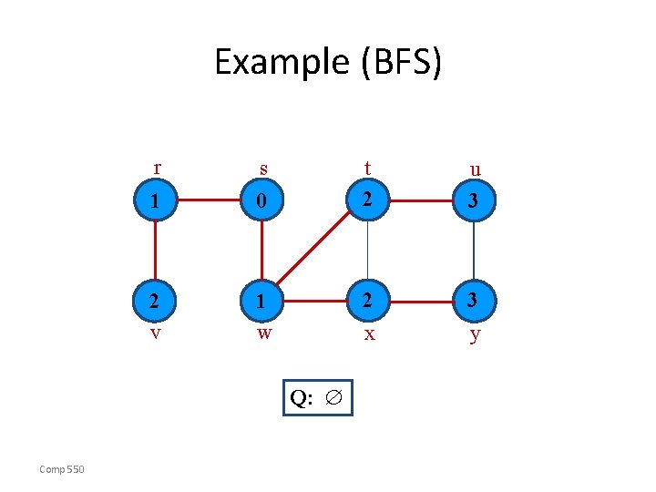
Example (BFS) r s 1 0 2 v 1 w u 3 2 3 y x Q: Comp 550 t 2

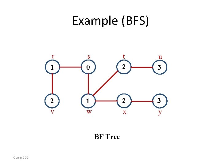
Example (BFS) r s 1 0 2 v 1 w u 3 2 3 y x BF Tree Comp 550 t 2

Analysis of BFS • Initialization takes O(V). • Traversal Loop – After initialization, each vertex is enqueued and dequeued at most once, and each operation takes O(1). So, total time for queuing is O(V). – The adjacency list of each vertex is scanned at most once. The sum of lengths of all adjacency lists is (E). • Summing up over all vertices => total running time of BFS is O(V+E), linear in the size of the adjacency list representation of graph. • Correctness Proof – We omit for BFS and DFS. – Will do for later algorithms. Comp 550

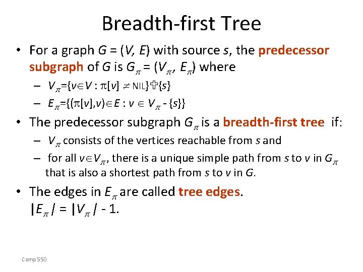
Breadth-first Tree • For a graph G = (V, E) with source s, the predecessor subgraph of G is G = (V , E ) where – V ={v V : [v] NIL} {s} – E ={( [v], v) E : v V - {s}} • The predecessor subgraph G is a breadth-first tree if: – V consists of the vertices reachable from s and – for all v V , there is a unique simple path from s to v in G that is also a shortest path from s to v in G. • The edges in E are called tree edges. |E | = |V | - 1. Comp 550

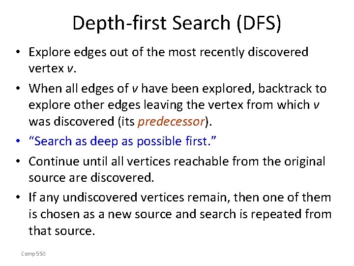
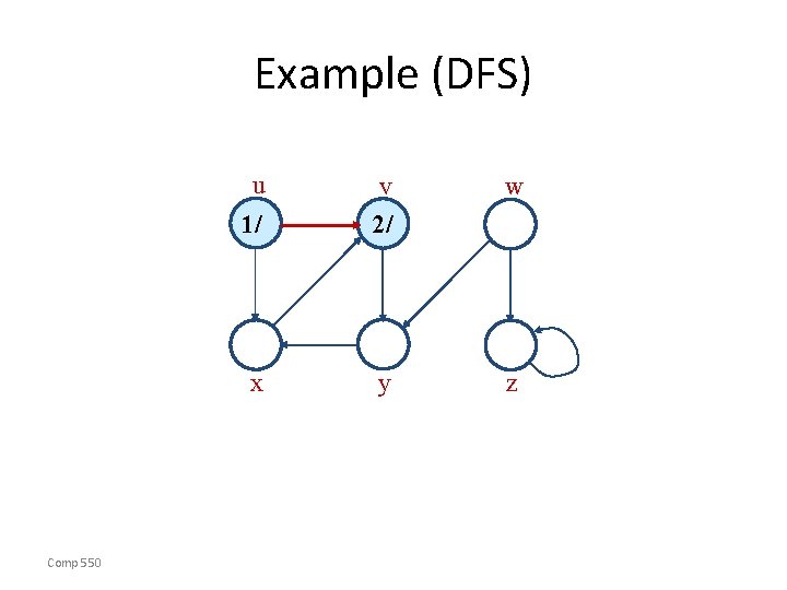
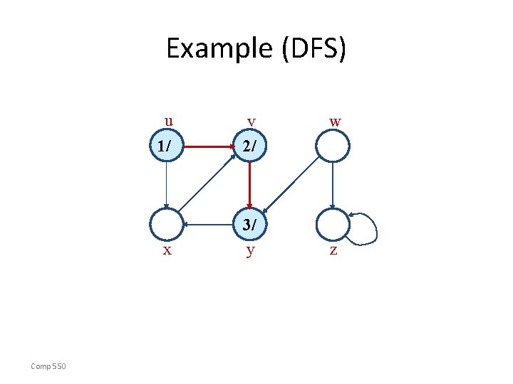
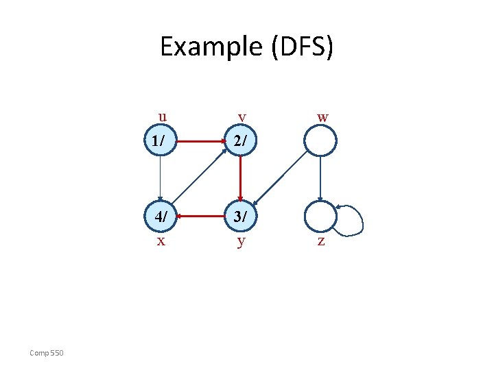
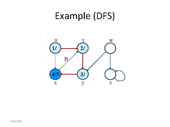
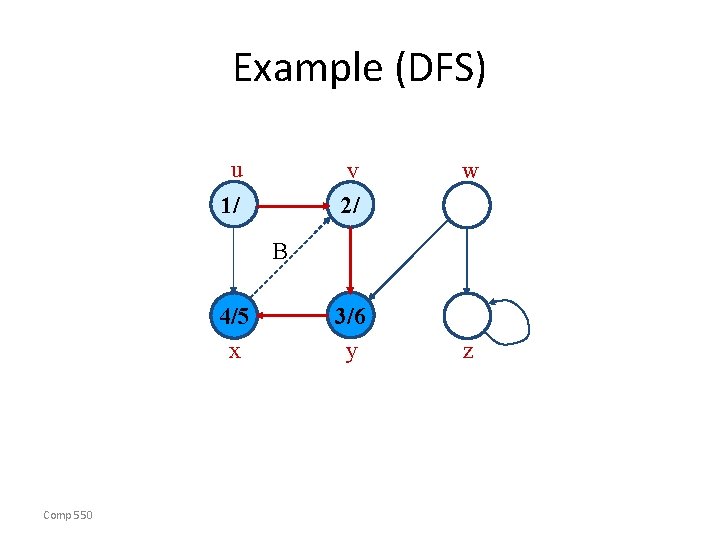
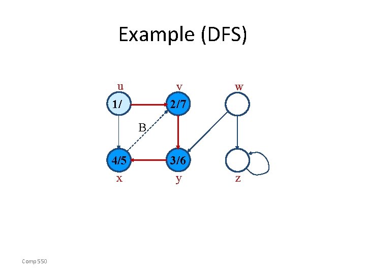
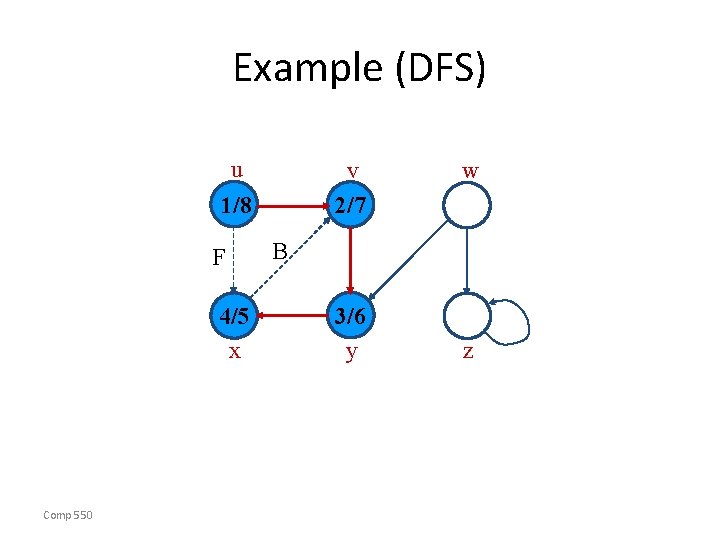
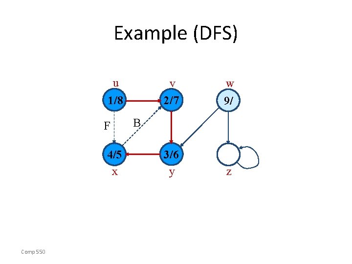
Depth-first Search (DFS) • Explore edges out of the most recently discovered vertex v. • When all edges of v have been explored, backtrack to explore other edges leaving the vertex from which v was discovered (its predecessor). • “Search as deep as possible first. ” • Continue until all vertices reachable from the original source are discovered. • If any undiscovered vertices remain, then one of them is chosen as a new source and search is repeated from that source. Comp 550

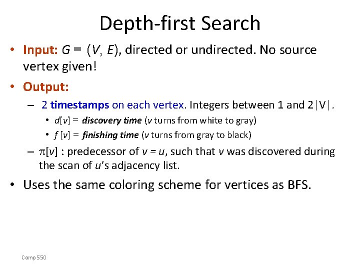
Depth-first Search • Input: G = (V, E), directed or undirected. No source vertex given! • Output: – 2 timestamps on each vertex. Integers between 1 and 2|V|. • d[v] = discovery time (v turns from white to gray) • f [v] = finishing time (v turns from gray to black) – [v] : predecessor of v = u, such that v was discovered during the scan of u’s adjacency list. • Uses the same coloring scheme for vertices as BFS. Comp 550

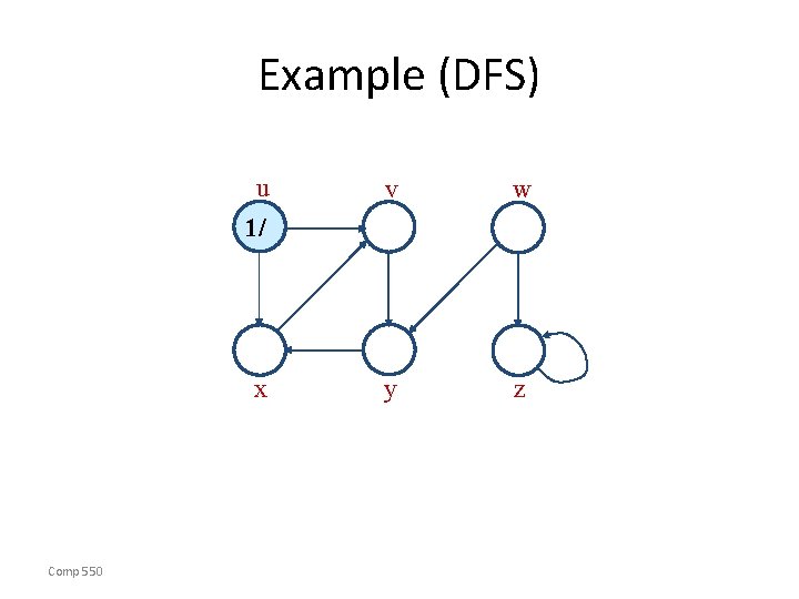
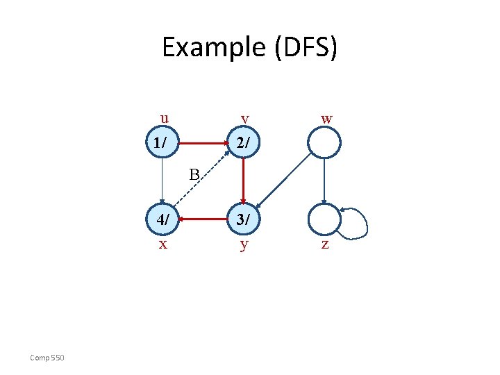
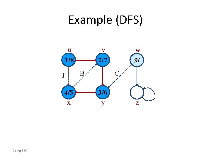
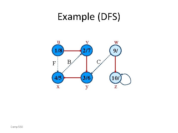
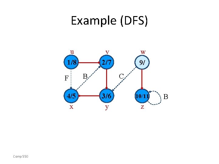
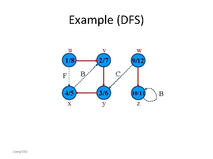
Pseudo-code DFS(G) 1. for each vertex u V[G] 2. do color[u] white 3. [u] NIL 4. time 0 5. for each vertex u V[G] 6. do if color[u] = white 7. then DFS-Visit(u) Uses a global timestamp time. Example: animation. Comp 550 DFS-Visit(u) 1. color[u] GRAY White vertex u has been discovered 2. time + 1 3. d[u] time 4. for each v Adj[u] 5. do if color[v] = WHITE 6. then [v] u 7. DFS-Visit(v) 8. color[u] BLACK Blacken u; it is finished. 9. f[u] time + 1

Example (DFS) u v w y z 1/ x Comp 550

Example (DFS) u Comp 550 w 1/ v 2/ x y z

Example (DFS) u Comp 550 1/ v 2/ x 3/ y w z

Example (DFS) u Comp 550 1/ v 2/ 4/ x 3/ y w z

Example (DFS) u v 2/ 1/ w B 4/ x Comp 550 3/ y z

Example (DFS) u v 2/ 1/ w B 4/5 x Comp 550 3/ y z

Example (DFS) u v 2/ 1/ w B 4/5 x Comp 550 3/6 y z

Example (DFS) u v 2/7 1/ w B 4/5 x Comp 550 3/6 y z

Example (DFS) u v 2/7 1/ F 4/5 x Comp 550 w B 3/6 y z

Example (DFS) u v 2/7 1/8 F 4/5 x Comp 550 w B 3/6 y z

Example (DFS) u 1/8 F 4/5 x Comp 550 v 2/7 w 9/ 3/6 y z B

Example (DFS) u v 2/7 1/8 F 4/5 x Comp 550 B w 9/ C 3/6 y z

Example (DFS) u v 2/7 1/8 F 4/5 x Comp 550 B w 9/ C 3/6 y 10/ z

Example (DFS) u v 2/7 1/8 F 4/5 x Comp 550 B w 9/ C 3/6 y 10/ z B

Example (DFS) u v 2/7 1/8 F 4/5 x Comp 550 B w 9/ C 3/6 y 10/11 z B

Example (DFS) u v 2/7 1/8 F 4/5 x Comp 550 B w 9/12 C 3/6 y 10/11 z B

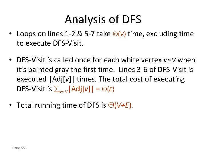
Analysis of DFS • Loops on lines 1 -2 & 5 -7 take (V) time, excluding time to execute DFS-Visit. • DFS-Visit is called once for each white vertex v V when it’s painted gray the first time. Lines 3 -6 of DFS-Visit is executed |Adj[v]| times. The total cost of executing DFS-Visit is v V|Adj[v]| = (E) • Total running time of DFS is (V+E). Comp 550

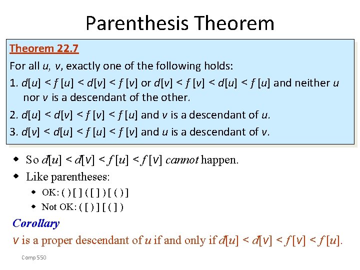
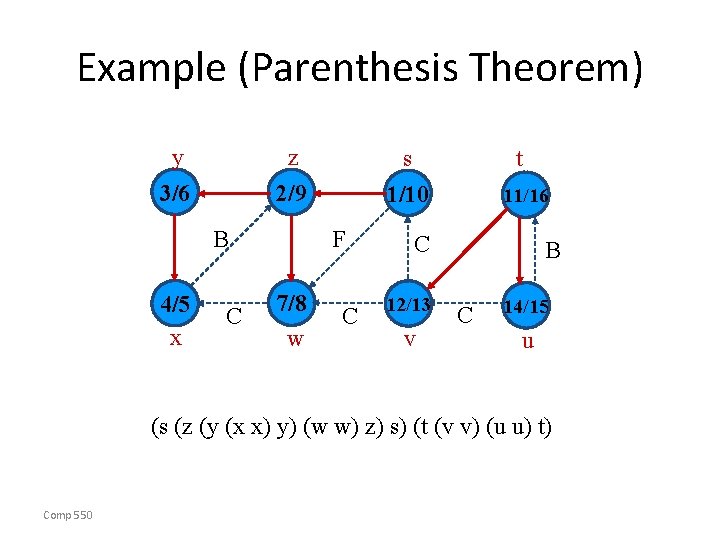
Parenthesis Theorem 22. 7 For all u, v, exactly one of the following holds: 1. d[u] < f [u] < d[v] < f [v] or d[v] < f [v] < d[u] < f [u] and neither u nor v is a descendant of the other. 2. d[u] < d[v] < f [u] and v is a descendant of u. 3. d[v] < d[u] < f [v] and u is a descendant of v. w So d[u] < d[v] < f [u] < f [v] cannot happen. w Like parentheses: w OK: ( ) [ ] ( [ ] ) [ ( ) ] w Not OK: ( [ ) ] [ ( ] ) Corollary v is a proper descendant of u if and only if d[u] < d[v] < f [u]. Comp 550

Example (Parenthesis Theorem) y z 2/9 3/6 B 4/5 x C F 7/8 w t s 1/10 C 11/16 C 12/13 v B C 14/15 u (s (z (y (x x) y) (w w) z) s) (t (v v) (u u) t) Comp 550

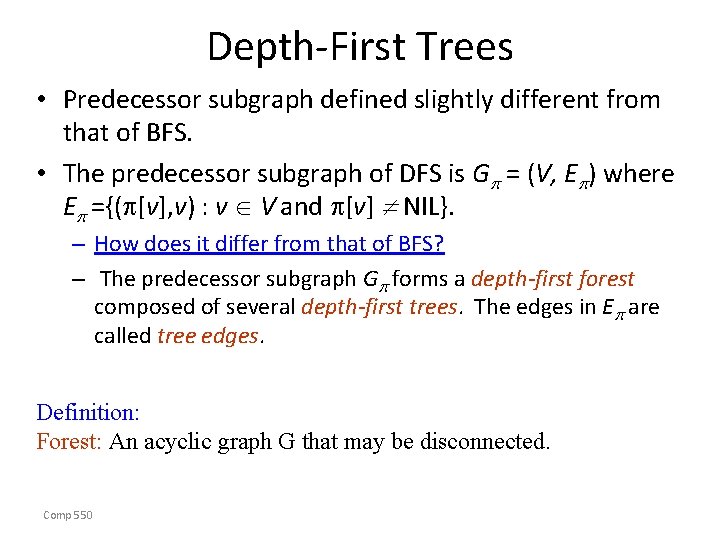
Depth-First Trees • Predecessor subgraph defined slightly different from that of BFS. • The predecessor subgraph of DFS is G = (V, E ) where E ={( [v], v) : v V and [v] NIL}. – How does it differ from that of BFS? – The predecessor subgraph G forms a depth-first forest composed of several depth-first trees. The edges in E are called tree edges. Definition: Forest: An acyclic graph G that may be disconnected. Comp 550

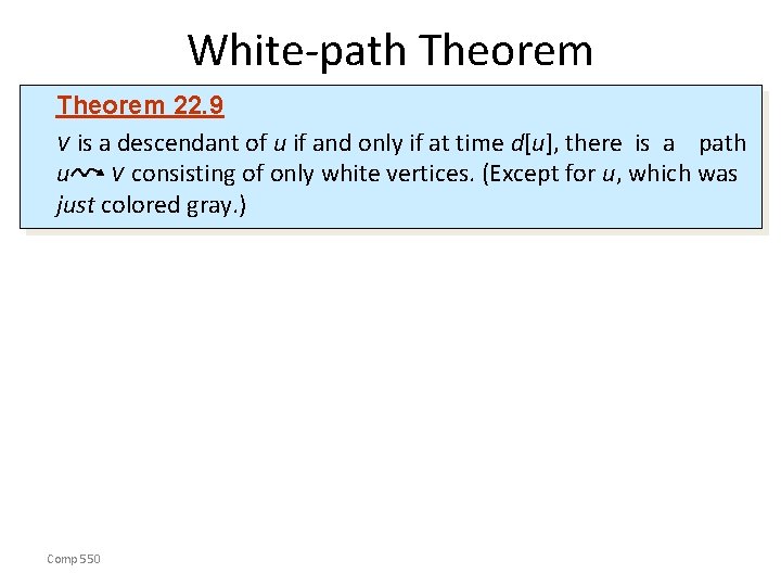
White-path Theorem 22. 9 v is a descendant of u if and only if at time d[u], there is a path u v consisting of only white vertices. (Except for u, which was just colored gray. ) Comp 550

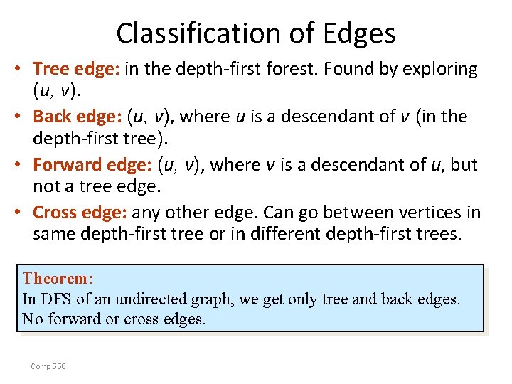
Classification of Edges • Tree edge: in the depth-first forest. Found by exploring (u, v). • Back edge: (u, v), where u is a descendant of v (in the depth-first tree). • Forward edge: (u, v), where v is a descendant of u, but not a tree edge. • Cross edge: any other edge. Can go between vertices in same depth-first tree or in different depth-first trees. Theorem: In DFS of an undirected graph, we get only tree and back edges. No forward or cross edges. Comp 550