Graph Algorithms Breadth First Depth First Search Network
Graph Algorithms Breadth First & Depth First Search
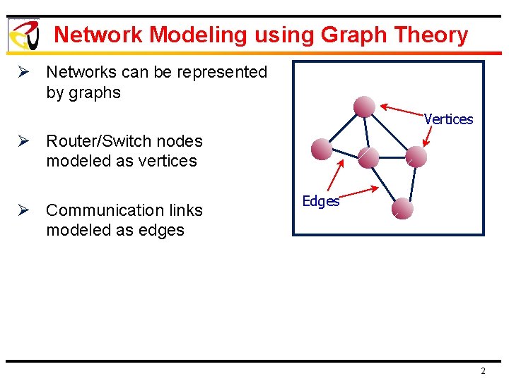
Network Modeling using Graph Theory Ø Networks can be represented by graphs Vertices Ø Router/Switch nodes modeled as vertices Ø Communication links modeled as edges Edges 2
Basic Concepts/Definitions Graph – A Graph is defined as a set of: Ø V = Nodes (vertices) Ø E = Edges (links, arcs) between pairs of nodes Ø Denoted by G = (V, E). Ø Graph Size Parameters: Ø Order of G: number of vertices, n = |V|, Ø Size of G: number of edges, m = |E|. Ø The running time of algorithms are usually measured in terms of the order and size of a graph 3
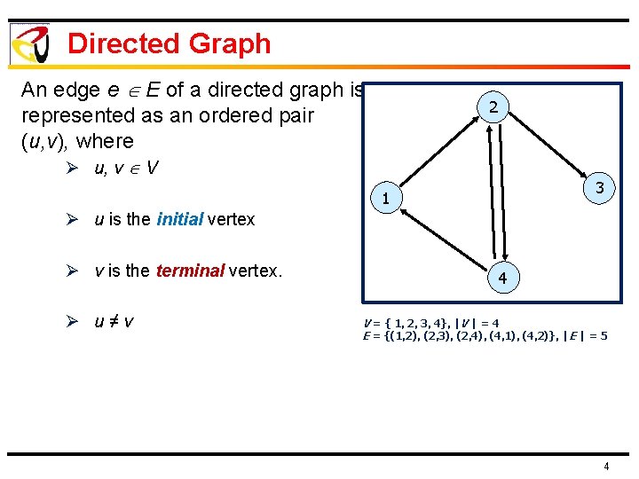
Directed Graph An edge e E of a directed graph is represented as an ordered pair (u, v), where 2 Ø u, v V 3 1 Ø u is the initial vertex Ø v is the terminal vertex. Ø u≠v 4 V = { 1, 2, 3, 4}, |V | = 4 E = {(1, 2), (2, 3), (2, 4), (4, 1), (4, 2)}, |E | = 5 4
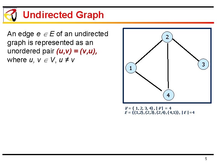
Undirected Graph An edge e E of an undirected graph is represented as an unordered pair (u, v) = (v, u), where u, v V, u ≠ v 2 3 1 4 V = { 1, 2, 3, 4}, |V | = 4 E = {(1, 2), (2, 3), (2, 4), (4, 1)}, |E |=4 5
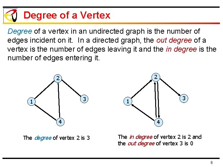
Degree of a Vertex Degree of a vertex in an undirected graph is the number of edges incident on it. In a directed graph, the out degree of a vertex is the number of edges leaving it and the in degree is the number of edges entering it. 2 2 3 1 4 The degree of vertex 2 is 3 3 1 4 The in degree of vertex 2 is 2 and the out degree of vertex 3 is 0 6
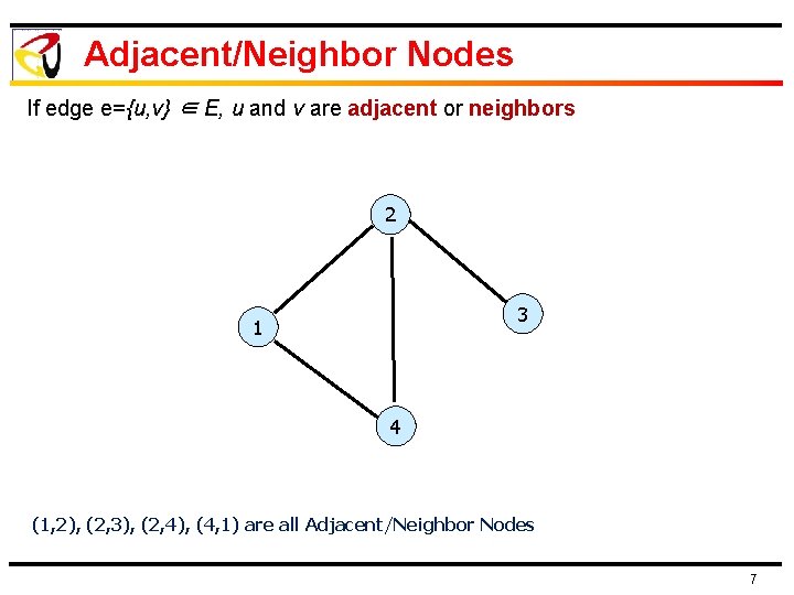
Adjacent/Neighbor Nodes If edge e={u, v} ∈ E, u and v are adjacent or neighbors 2 3 1 4 (1, 2), (2, 3), (2, 4), (4, 1) are all Adjacent/Neighbor Nodes 7
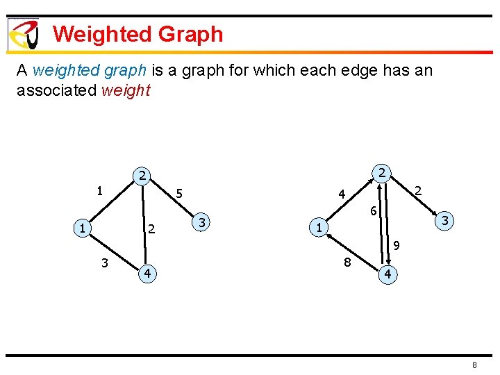
Weighted Graph A weighted graph is a graph for which each edge has an associated weight 2 2 1 1 5 2 2 4 3 6 3 1 9 3 4 8
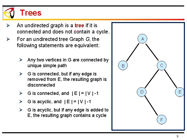
Trees Ø Ø An undirected graph is a tree if it is connected and does not contain a cycle. For an undirected tree Graph G, the following statements are equivalent: Ø Any two vertices in G are connected by unique simple path A C B Ø G is connected, but if any edge is removed from E, the resulting graph is disconnected Ø G is connected, and | E | = | V | -1 D E Ø G is acyclic, and | E | = | V | -1 Ø G is acyclic, but if any edge is added to E, the resulting graph contains a cycle F 9
Graph Representation: Adjacency Matrix l 10
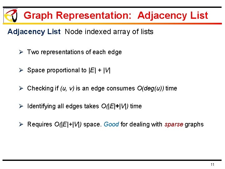
Graph Representation: Adjacency List Node indexed array of lists Ø Two representations of each edge Ø Space proportional to |E| + |V| Ø Checking if (u, v) is an edge consumes O(deg(u)) time Ø Identifying all edges takes O(|E|+|V|) time Ø Requires O(|E|+|V|) space. Good for dealing with sparse graphs 11
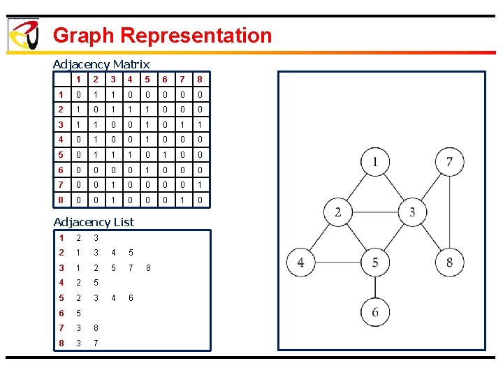
Graph Representation Adjacency Matrix 1 2 3 4 5 6 7 8 1 0 1 1 0 0 0 2 1 0 1 1 1 0 0 0 3 1 1 0 0 1 1 4 0 1 0 0 0 5 0 1 1 1 0 0 6 0 0 1 0 0 0 7 0 0 1 8 0 0 1 0 Adjacency List 1 2 3 2 1 3 4 5 3 1 2 5 7 4 2 5 5 2 3 4 6 6 5 7 3 8 8 3 7 8
Graph Searching Algorithms Ø Breadth-First Search (BFS) Ø Depth-First Search (DFS) 13
Breadth-First Search l 14
Breadth-First Search Vertices Coloring Ø White: Undiscovered Ø Gray: Discovered but not Finished Ø Black: Finished (All adjacent vertices discovered) 15
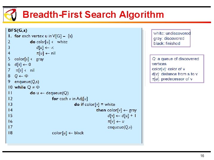
Breadth-First Search Algorithm 16
![Example 3 2 1 6 4 5 7 8 Q v d[v] 1 0 Example 3 2 1 6 4 5 7 8 Q v d[v] 1 0](http://slidetodoc.com/presentation_image_h2/99b495e69bbcdddd4239d47ef566dc9f/image-17.jpg)
Example 3 2 1 6 4 5 7 8 Q v d[v] 1 0 17
![Example 3 2 1 6 4 5 7 8 Q v d[v] 2 6 Example 3 2 1 6 4 5 7 8 Q v d[v] 2 6](http://slidetodoc.com/presentation_image_h2/99b495e69bbcdddd4239d47ef566dc9f/image-18.jpg)
Example 3 2 1 6 4 5 7 8 Q v d[v] 2 6 7 1 18
![Example 3 2 1 6 4 5 7 8 Q v d[v] 6 7 Example 3 2 1 6 4 5 7 8 Q v d[v] 6 7](http://slidetodoc.com/presentation_image_h2/99b495e69bbcdddd4239d47ef566dc9f/image-19.jpg)
Example 3 2 1 6 4 5 7 8 Q v d[v] 6 7 3 1 1 2 19
![Example 3 2 1 6 4 5 7 8 Q v d[v] 7 3 Example 3 2 1 6 4 5 7 8 Q v d[v] 7 3](http://slidetodoc.com/presentation_image_h2/99b495e69bbcdddd4239d47ef566dc9f/image-20.jpg)
Example 3 2 1 6 4 5 7 8 Q v d[v] 7 3 5 1 2 2 20
![Example 3 2 1 6 4 5 7 8 Q v d[v] 3 5 Example 3 2 1 6 4 5 7 8 Q v d[v] 3 5](http://slidetodoc.com/presentation_image_h2/99b495e69bbcdddd4239d47ef566dc9f/image-21.jpg)
Example 3 2 1 6 4 5 7 8 Q v d[v] 3 5 8 2 21
![Example 3 2 1 6 4 5 7 8 Q v d[v] 5 8 Example 3 2 1 6 4 5 7 8 Q v d[v] 5 8](http://slidetodoc.com/presentation_image_h2/99b495e69bbcdddd4239d47ef566dc9f/image-22.jpg)
Example 3 2 1 6 4 5 7 8 Q v d[v] 5 8 2 2 22
![Example 3 2 1 6 4 5 7 8 Q v d[v] 8 4 Example 3 2 1 6 4 5 7 8 Q v d[v] 8 4](http://slidetodoc.com/presentation_image_h2/99b495e69bbcdddd4239d47ef566dc9f/image-23.jpg)
Example 3 2 1 6 4 5 7 8 Q v d[v] 8 4 2 3 23
![Example 3 2 1 6 4 5 7 8 Q v d[v] 4 3 Example 3 2 1 6 4 5 7 8 Q v d[v] 4 3](http://slidetodoc.com/presentation_image_h2/99b495e69bbcdddd4239d47ef566dc9f/image-24.jpg)
Example 3 2 1 6 4 5 7 8 Q v d[v] 4 3 24
![Example 3 2 1 6 4 5 7 8 Q v d[v] 25 Example 3 2 1 6 4 5 7 8 Q v d[v] 25](http://slidetodoc.com/presentation_image_h2/99b495e69bbcdddd4239d47ef566dc9f/image-25.jpg)
Example 3 2 1 6 4 5 7 8 Q v d[v] 25
![Example: Resultant BFS Tree d[v]=1 π[v]=1 3 2 1 d[v]=2 π[v]=2 d[v]=1 π[v]=1 6 Example: Resultant BFS Tree d[v]=1 π[v]=1 3 2 1 d[v]=2 π[v]=2 d[v]=1 π[v]=1 6](http://slidetodoc.com/presentation_image_h2/99b495e69bbcdddd4239d47ef566dc9f/image-26.jpg)
Example: Resultant BFS Tree d[v]=1 π[v]=1 3 2 1 d[v]=2 π[v]=2 d[v]=1 π[v]=1 6 d[v]=2 π[v]=6 4 d[v]=3 π[v]=5 5 7 8 d[v]=2 π[v]=7 d[v]=1 π[v]=1 26
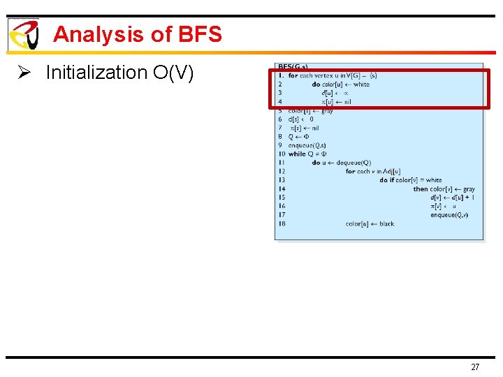
Analysis of BFS Ø Initialization O(V) 27
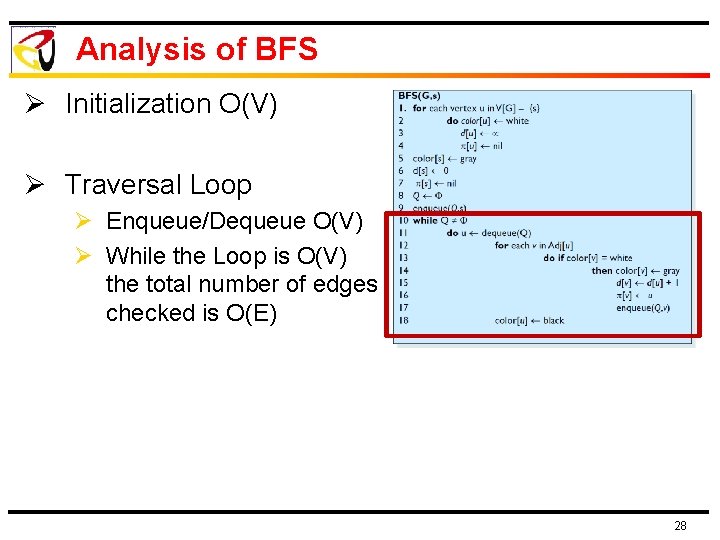
Analysis of BFS Ø Initialization O(V) Ø Traversal Loop Ø Enqueue/Dequeue O(V) Ø While the Loop is O(V) the total number of edges checked is O(E) 28
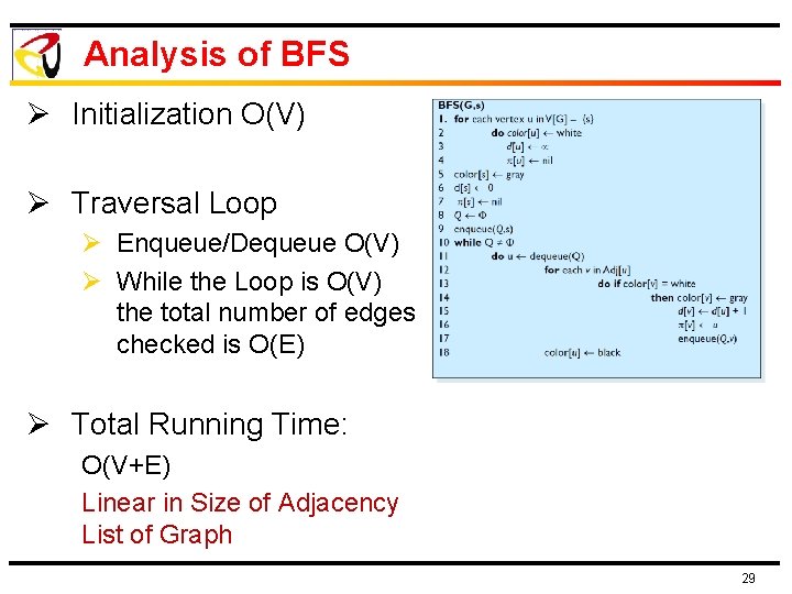
Analysis of BFS Ø Initialization O(V) Ø Traversal Loop Ø Enqueue/Dequeue O(V) Ø While the Loop is O(V) the total number of edges checked is O(E) Ø Total Running Time: O(V+E) Linear in Size of Adjacency List of Graph 29
Depth-First Search Ø Explore edges out of the most recently discovered vertex v Ø When all edges of v have been explored, back track to explore other edges from the predecessor of v Ø Search as Deep as Possible 30
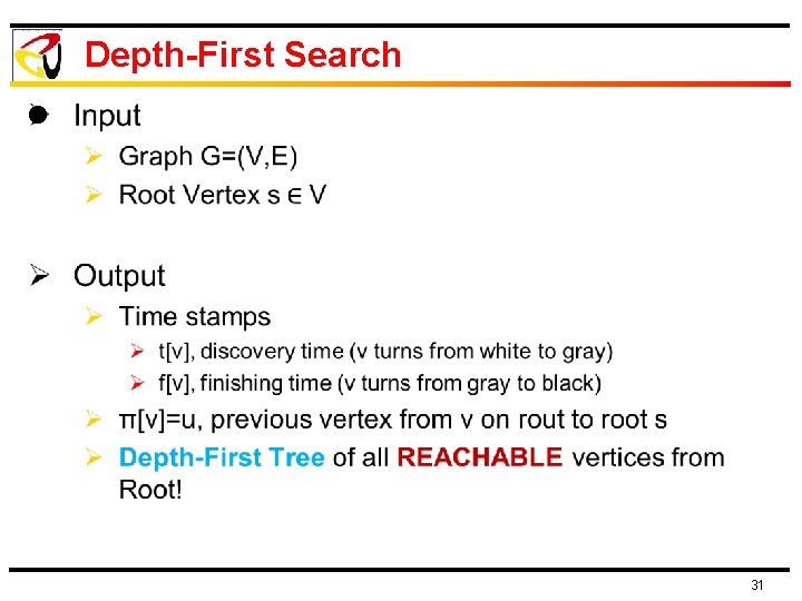
Depth-First Search l 31
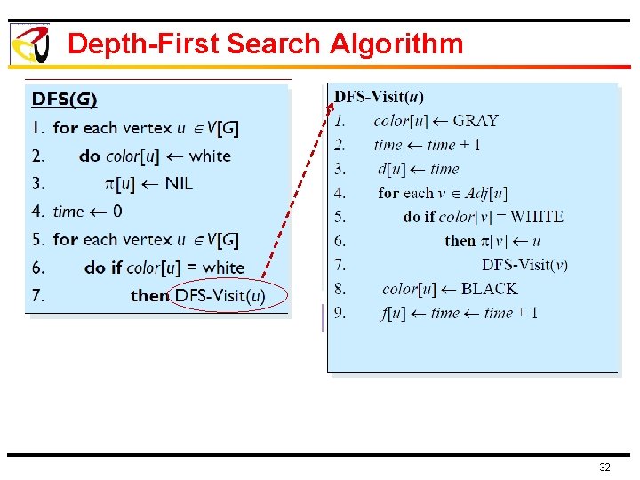
Depth-First Search Algorithm 32
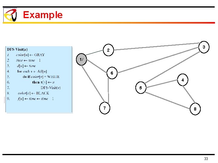
Example 3 2 1/ 6 4 5 7 8 33
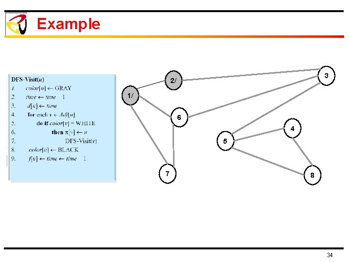
Example 3 2/ 1/ 6 4 5 7 8 34
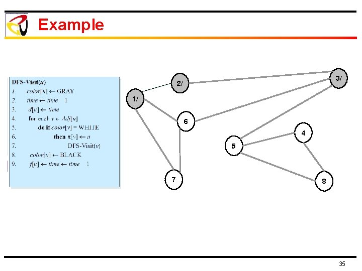
Example 3/ 2/ 1/ 6 4 5 7 8 35
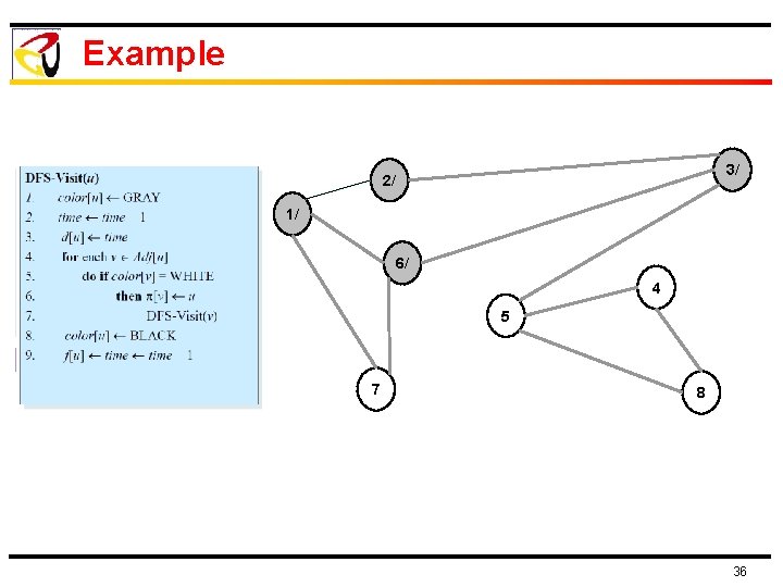
Example 3/ 2/ 1/ 6/ 4 5 7 8 36
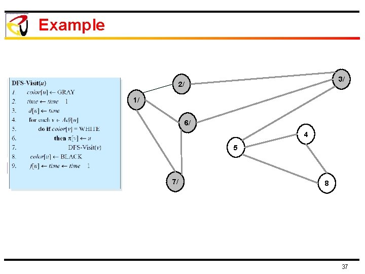
Example 3/ 2/ 1/ 6/ 4 5 7/ 8 37
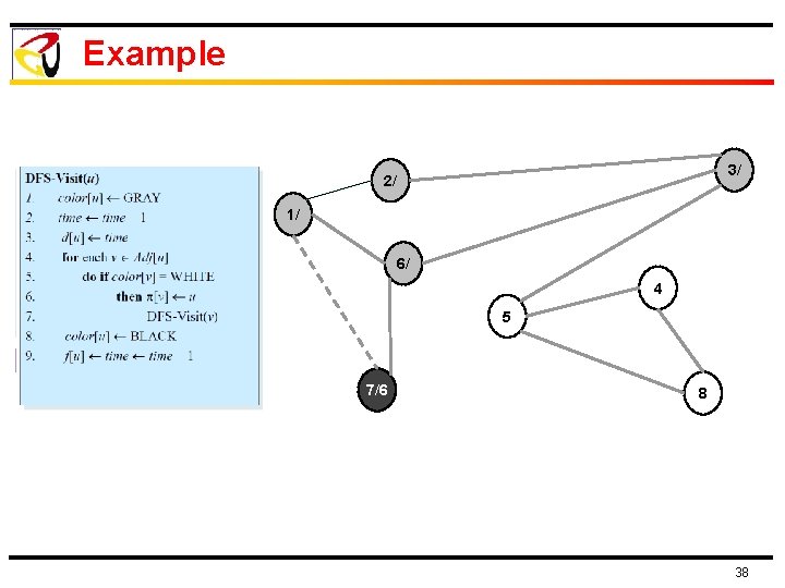
Example 3/ 2/ 1/ 6/ 4 5 7/6 8 38
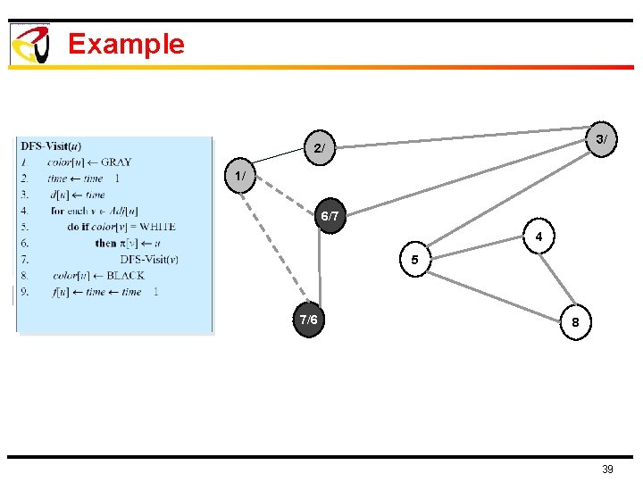
Example 3/ 2/ 1/ 6/7 4 5 7/6 8 39
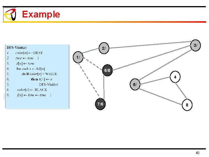
Example 3/ 2/ 1/ 6/8 4 5/ 7/6 8 40
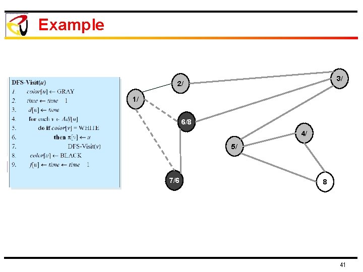
Example 3/ 2/ 1/ 6/8 4/ 5/ 7/6 8 41
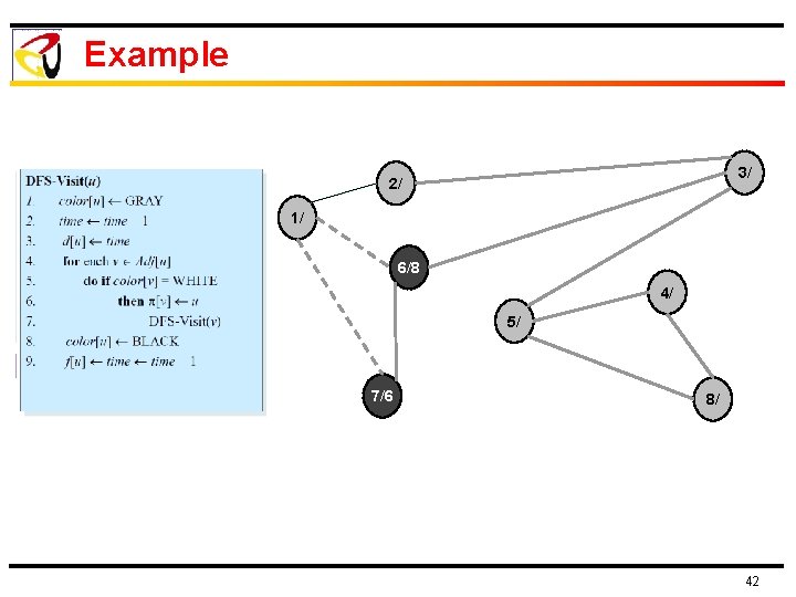
Example 3/ 2/ 1/ 6/8 4/ 5/ 7/6 8/ 42
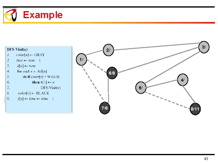
Example 3/ 2/ 1/ 6/8 4/ 5/ 7/6 8/11 43
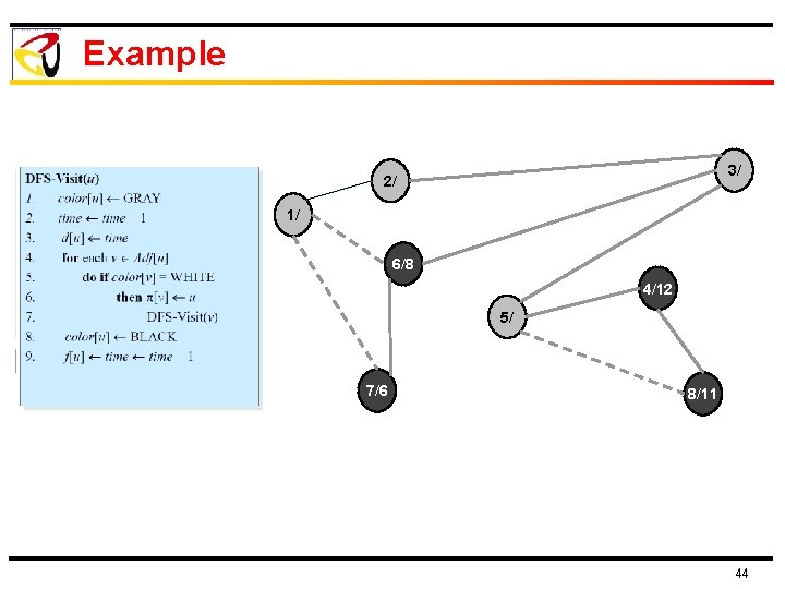
Example 3/ 2/ 1/ 6/8 4/12 5/ 7/6 8/11 44
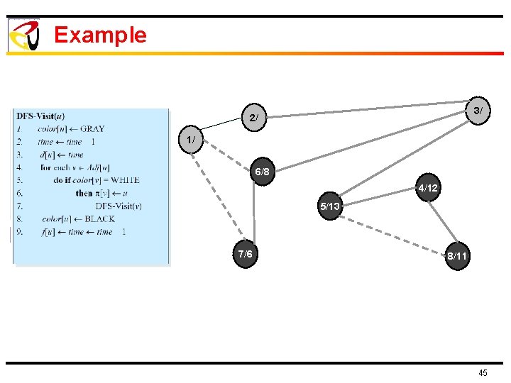
Example 3/ 2/ 1/ 6/8 4/12 5/13 7/6 8/11 45
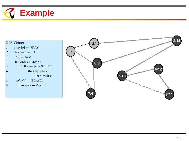
Example 3/14 2/ 1/ 6/8 4/12 5/13 7/6 8/11 46
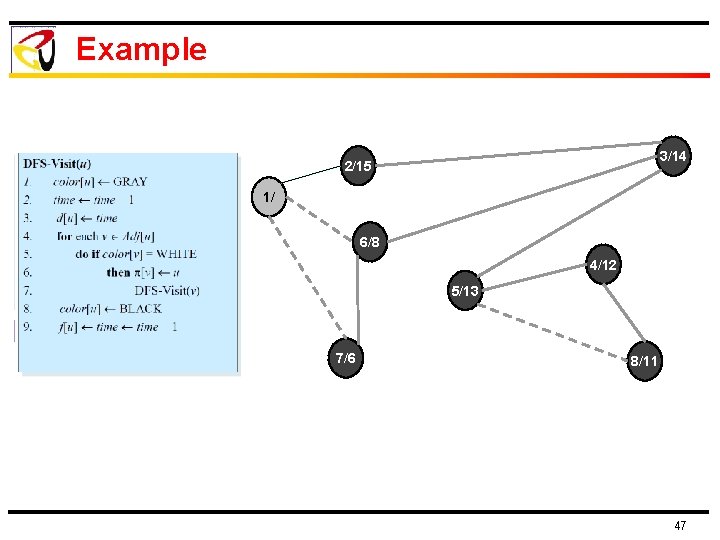
Example 3/14 2/15 1/ 6/8 4/12 5/13 7/6 8/11 47
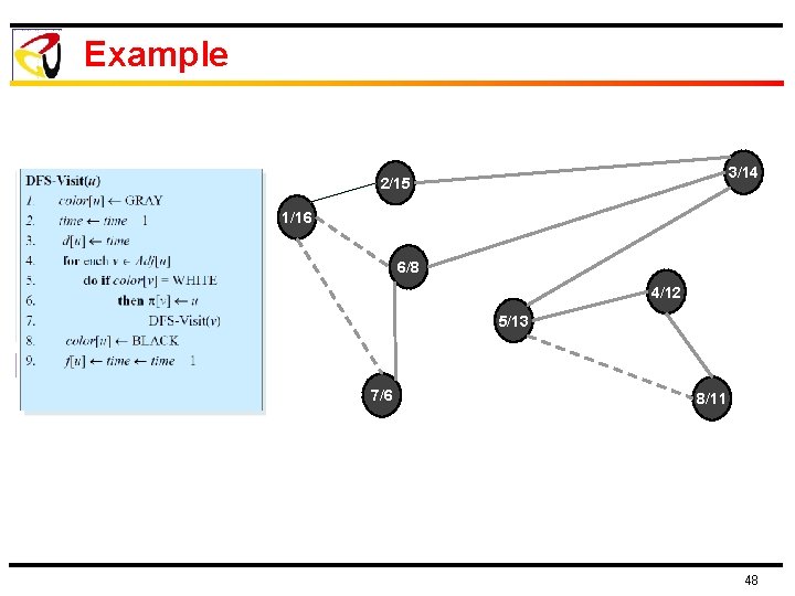
Example 3/14 2/15 1/16 6/8 4/12 5/13 7/6 8/11 48
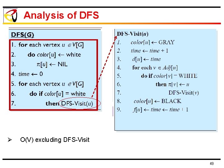
Analysis of DFS Ø O(V) excluding DFS-Visit 49
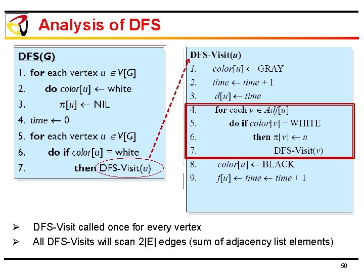
Analysis of DFS Ø Ø DFS-Visit called once for every vertex All DFS-Visits will scan 2|E| edges (sum of adjacency list elements) 50
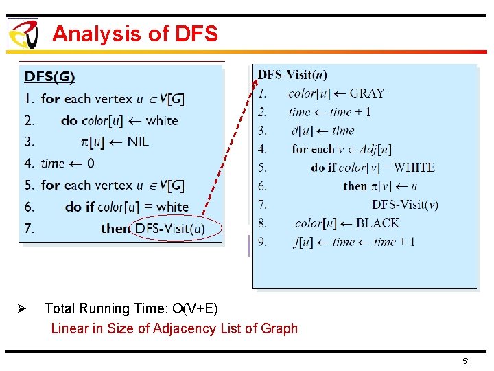
Analysis of DFS Ø Total Running Time: O(V+E) Linear in Size of Adjacency List of Graph 51
- Slides: 51