Granulated Activated Carbon Filter Model Simulations Razvan Carbunescu

Granulated Activated Carbon Filter Model & Simulations Razvan Carbunescu Sarah Johnston Mona Crump Brett Mc. Cullough Daniel Guidry

What is GAC? GAC stands for Granular Activated Carbon ¡ It is a low volume, high surface area material ¡ The carbon based material is converted to activated carbon by thermal decomposition in a furnace using a controlled atmosphere and heat. ¡

GAC Filter Description The Glass beads and wool evenly disperse air flow. ¡ A syringe pump empties pollutants into the air supply. ¡

GAC Properties – Adsorption ¡ ¡ ¡ The pores in activated carbon result in a large surface area. A gram of activated carbon can have a surface area of 500 to 1500 meters squared. One pound of GAC, about a quart in volume, can have a total surface area of 125 acres

Biofilter Considerations • Biofilters are sensitive to Input loading. • Too much or too little load can disrupt the effectiveness of the biofilter. • GAC filters can help to alleviate drastic oscillations in biofilter input loading by providing a steady load.

Providing a Steady State Input to the Biofilter For Example: 500 ppm factory output 1000 ppm “shock loading” factory output 0 ppm (notypical load) median factory output passes load through at biofilter same level reduces excess load to GAC releases stored contaminant 500 ppm GAC output / Biofilter input

Equations – Mobile Phase

Equations – Pore Phase

Equations – Non-linear equation 1. 3 The non-linear coupling equation

Matrix Approximations ¡ We use MATLAB to calculate the matrices needed to approximate the functions ¡ More Legendre roots means a better approximation for the derivatives and a better approximation for the general functions ¡ Legendre Roots are given from the tables by Stroud and Secrest(1966) up to thirty significant digits

Matrix Approximations ¡ ¡ Radial – symmetric, spherical geometry Used to approximate the carbon beads themselves W= B= ( 0. 0098 ( -62. 623 22. 579 -3. 984 1. 5827 -0. 98636 0. 90471 46. 257 ( 0. 09491 ( -15. 66996 9. 96512 26. 93285 0. 0349 80. 052 -82. 222 41. 6 -10. 166 5. 3578 -4. 578 -195. 81 0. 19081 0. 04762 ) 20. 03488 -44. 33004 -86. 9329 0. 0635 -25. 737 75. 799 -109. 32 70. 264 -22. 169 15. 942 488. 51 0. 0819 13. 188 -23. 892 90. 627 -166. 99 136. 52 -59. 671 -1024. 6 -4. 36492 34. 36492 60. 00000 0. 0796 -7. 9903 12. 242 -27. 8 132. 72 -322. 49 377. 01 2044. 8 ) 0. 0541 0. 0095 ) 4. 9756 -7. 1015 13. 572 -39. 386 255. 95 -1024. 3 -3127. 2 -1. 8647 2. 5966 -4. 6954 11. 975 -52. 178 694. 74 1768 )

Matrix Approximations ¡ ¡ Axial – non-symmetric, planar geometry Used to approximate the flow itself A= A= ( -43. 0014 -18. 2773 5. 2138 -2. 6370 1. 6212 -1. 0631 0. 6385 -0. 9997 47. 9927 14. 2907 -10. 5516 4. 6889 -2. 7784 1. 7956 -1. 0720 1. 6765 -6. 6848 5. 1519 2. 3498 -5. 3795 2. 5267 -1. 5120 0. 8766 -1. 3628 ( -3 -1 1 4 0 -4 2. 6155 -1. 7720 4. 1637 0. 5063 -4. 1912 1. 9549 -1. 0495 1. 6079 -1 1 3 ) -1. 6079 1. 0498 -1. 9552 4. 1903 -0. 5051 -4. 1617 1. 7711 -2. 6155 1. 3628 -1. 6765 -0. 8770 1. 0728 1. 5125 -1. 7966 -2. 5266 2. 7791 5. 3799 -4. 6911 -2. 3548 10. 5570 -5. 1525 -14. 2884 6. 6848 -47. 9927 0. 9997 -0. 6389 1. 0636 -1. 6215 2. 6381 -5. 2158 18. 2761 43. 0014 )

Legendre Roots ¡ Axial roots for non-symetric planar geometry now calculated ¡ Radial roots not necessary for calculations ¡ Matlab program solves for the roots of the equations after polynomial is formed ¡ Limited to 80 roots for non-symmetric and 40 roots for symmetric because of the size of the polynomial coeficients

New GAC Filter Interface ¡ Based on the old interface combined with the matlab program ¡ Integrates the resulting graph into the interfcace ¡ Allows for modification of the discretization accuracy ¡ Has initial parameters set

New GAC Filter Interface (cont) ¡ Allows for the specification if the input concentration from an external excel file ¡ Allows for specification of the type of input concentration (steady, intermitent, …) ¡ Allows for the results of the simulation to be saved to an excel file for later use ¡ Allows for adding an experimental data set to the graph to compare results

New GAC Filter Interface (cont)

3 Axial Points 3 Radial Points ¡ Comparison of experimental results versus simulation results with 3 axial points and 3 radial points

5 Axial Points 3 Radial Points ¡ Comparison of experimental results versus simulation results with 5 axial points and 3 radial points

7 Axial Points 3 Radial Points ¡ Comparison of experimental results versus simulation results with 7 axial points and 3 radial points

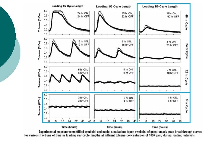
Intermittent vs. Continuous Loading

Questions?