Graham Hesketh Information Engineering Group RollsRoyce Strategic Research

Graham Hesketh Information Engineering Group Rolls-Royce Strategic Research Centre 6 July 2000 NCAF Manchester 2000 1

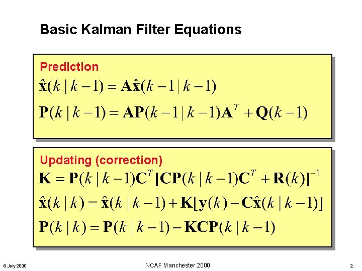
Basic Kalman Filter Equations Prediction Updating (correction) 6 July 2000 NCAF Manchester 2000 2

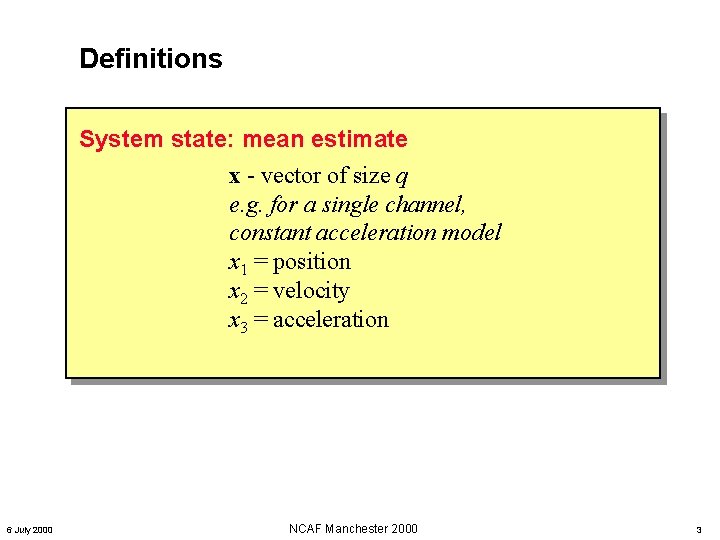
Definitions System state: mean estimate x - vector of size q e. g. for a single channel, constant acceleration model x 1 = position x 2 = velocity x 3 = acceleration 6 July 2000 NCAF Manchester 2000 3

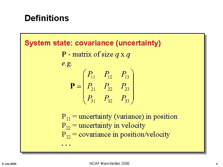
Definitions System state: covariance (uncertainty) P - matrix of size q x q e. g. P 11 = uncertainty (variance) in position P 22 = uncertainty in velocity P 12 = covariance in position/velocity. . . 6 July 2000 NCAF Manchester 2000 4

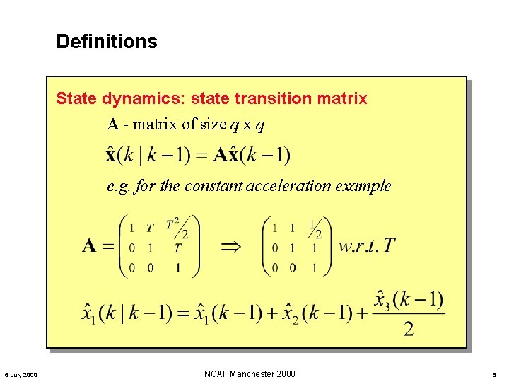
Definitions State dynamics: state transition matrix A - matrix of size q x q e. g. for the constant acceleration example 6 July 2000 NCAF Manchester 2000 5

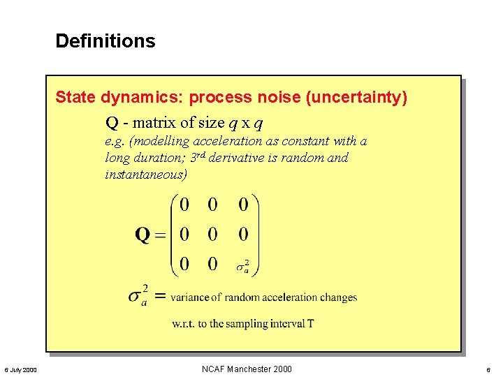
Definitions State dynamics: process noise (uncertainty) Q - matrix of size q x q e. g. (modelling acceleration as constant with a long duration; 3 rd derivative is random and instantaneous) 6 July 2000 NCAF Manchester 2000 6

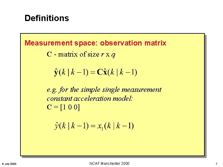
Definitions Measurement space: observation matrix C - matrix of size r x q e. g. for the simple single measurement constant acceleration model: C = [1 0 0] 6 July 2000 NCAF Manchester 2000 7

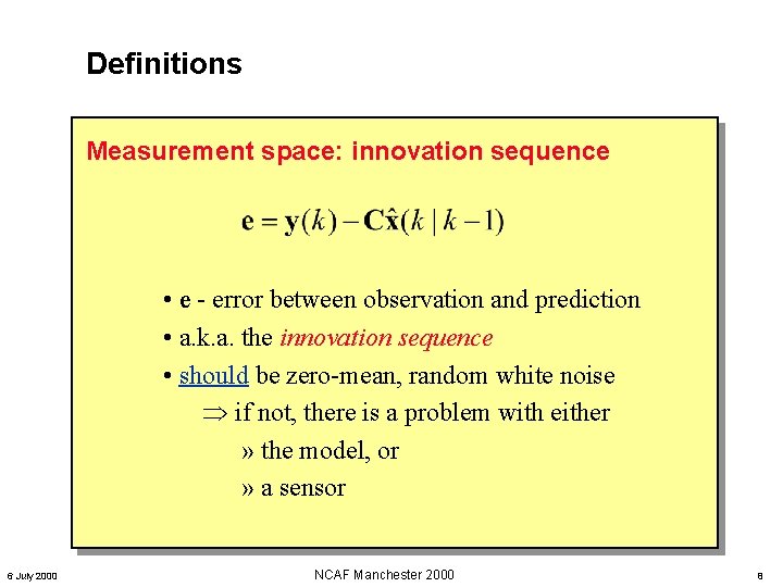
Definitions Measurement space: innovation sequence • e - error between observation and prediction • a. k. a. the innovation sequence • should be zero-mean, random white noise Þ if not, there is a problem with either » the model, or » a sensor 6 July 2000 NCAF Manchester 2000 8

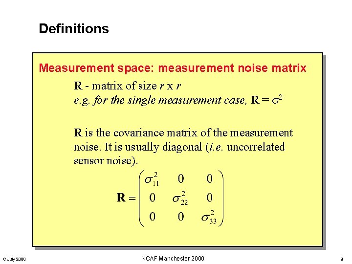
Definitions Measurement space: measurement noise matrix R - matrix of size r x r e. g. for the single measurement case, R = 2 R is the covariance matrix of the measurement noise. It is usually diagonal (i. e. uncorrelated sensor noise). 6 July 2000 NCAF Manchester 2000 9

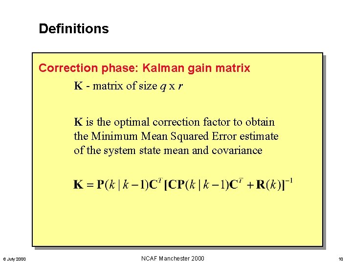
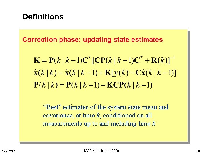
Definitions Correction phase: Kalman gain matrix K - matrix of size q x r K is the optimal correction factor to obtain the Minimum Mean Squared Error estimate of the system state mean and covariance 6 July 2000 NCAF Manchester 2000 10

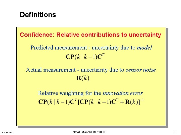
Definitions Confidence: Relative contributions to uncertainty Predicted measurement - uncertainty due to model Actual measurement - uncertainty due to sensor noise Relative weighting for the innovation error 6 July 2000 NCAF Manchester 2000 11

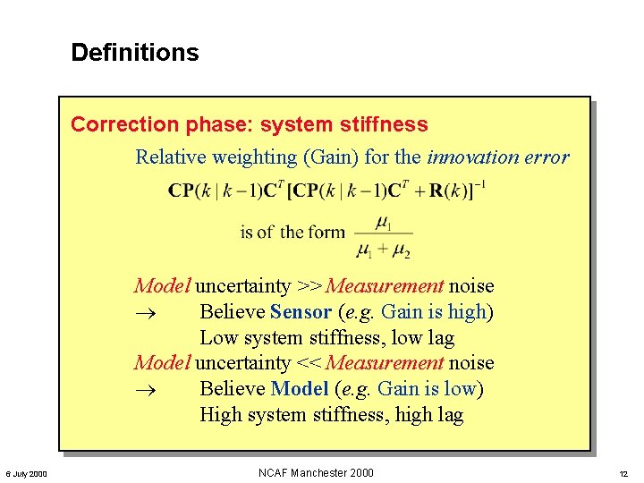
Definitions Correction phase: system stiffness Relative weighting (Gain) for the innovation error Model uncertainty >> Measurement noise Believe Sensor (e. g. Gain is high) Low system stiffness, low lag Model uncertainty << Measurement noise Believe Model (e. g. Gain is low) High system stiffness, high lag 6 July 2000 NCAF Manchester 2000 12

Definitions Correction phase: updating state estimates “Best” estimates of the system state mean and covariance, at time k, conditioned on all measurements up to and including time k 6 July 2000 NCAF Manchester 2000 13

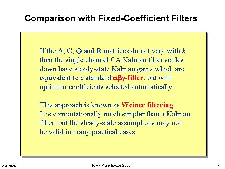
Comparison with Fixed-Coefficient Filters If the A, C, Q and R matrices do not vary with k then the single channel CA Kalman filter settles down have steady-state Kalman gains which are equivalent to a standard -filter, but with optimum coefficients selected automatically. This approach is known as Weiner filtering. It is computationally much simpler than a Kalman filter, but the steady-state assumptions may not be valid in many practical cases. 6 July 2000 NCAF Manchester 2000 14

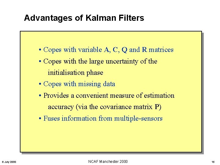
Advantages of Kalman Filters • Copes with variable A, C, Q and R matrices • Copes with the large uncertainty of the initialisation phase • Copes with missing data • Provides a convenient measure of estimation accuracy (via the covariance matrix P) • Fuses information from multiple-sensors 6 July 2000 NCAF Manchester 2000 15

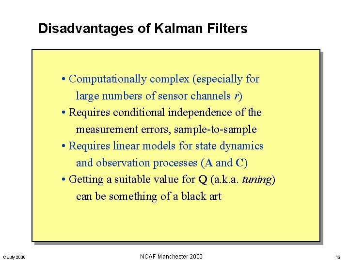
Disadvantages of Kalman Filters • Computationally complex (especially for large numbers of sensor channels r) • Requires conditional independence of the measurement errors, sample-to-sample • Requires linear models for state dynamics and observation processes (A and C) • Getting a suitable value for Q (a. k. a. tuning) can be something of a black art 6 July 2000 NCAF Manchester 2000 16

Dealing with the disadvantages [1] • Computationally complex (especially for large numbers of sensor channels r) Computers are getting faster all the time New algorithms for fast matrix inversion 6 July 2000 NCAF Manchester 2000 17

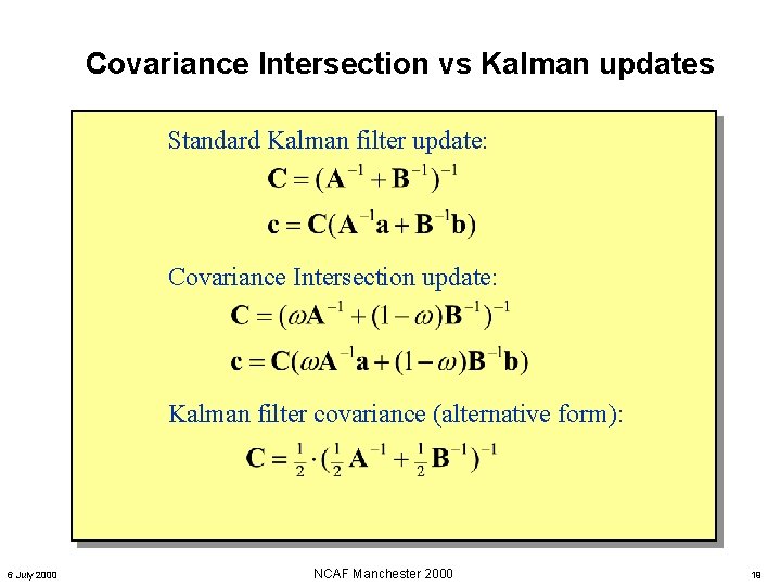
Dealing with the disadvantages [2] • Requires conditional independence of the measurement errors, sample-to-sample The independence criterion can be removed by using Covariance Intersection updating A B C a, b, c 6 July 2000 NCAF Manchester 2000 18

Covariance Intersection vs Kalman updates Standard Kalman filter update: Covariance Intersection update: Kalman filter covariance (alternative form): 6 July 2000 NCAF Manchester 2000 19

Dealing with the disadvantages [3] • Requires linear models for state dynamics and observation processes (A and C) This can be overcome by using the EKF (Extended Kalman Filter), but only at the expense of your sanity and all your free time A superior alternative to EKF is the Unscented Filter 6 July 2000 NCAF Manchester 2000 20

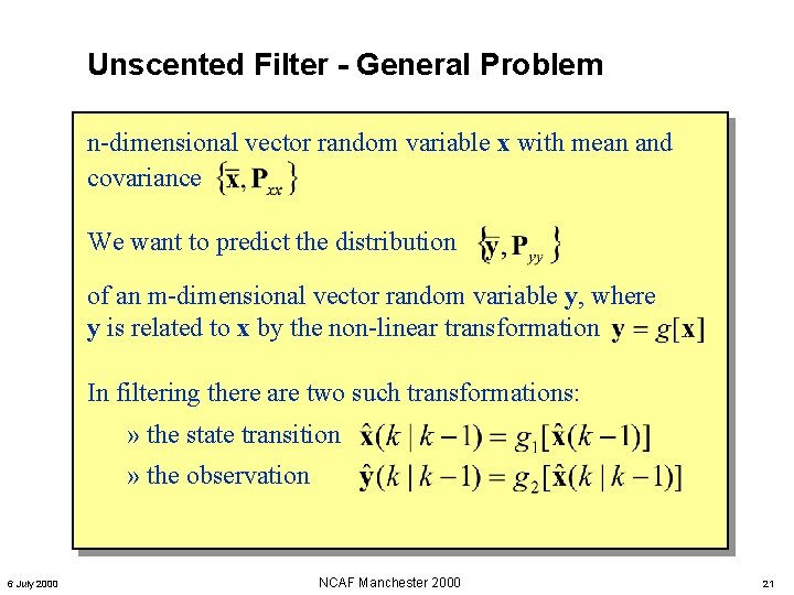
Unscented Filter - General Problem n-dimensional vector random variable x with mean and covariance We want to predict the distribution of an m-dimensional vector random variable y, where y is related to x by the non-linear transformation In filtering there are two such transformations: » the state transition » the observation 6 July 2000 NCAF Manchester 2000 21

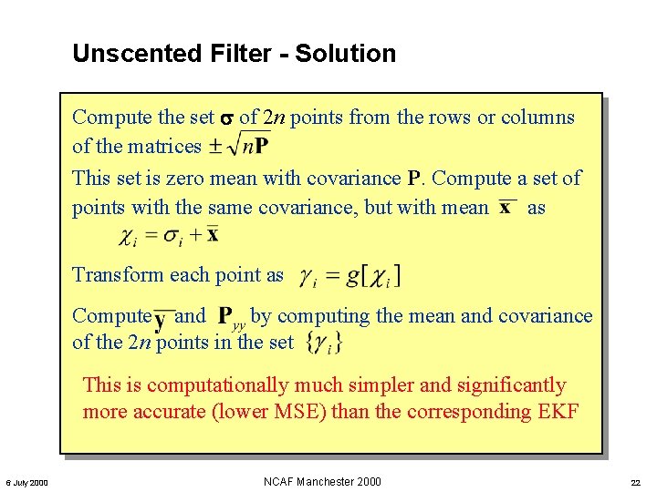
Unscented Filter - Solution Compute the set of 2 n points from the rows or columns of the matrices This set is zero mean with covariance P. Compute a set of points with the same covariance, but with mean as Transform each point as Compute and by computing the mean and covariance of the 2 n points in the set This is computationally much simpler and significantly more accurate (lower MSE) than the corresponding EKF 6 July 2000 NCAF Manchester 2000 22

Dealing with the disadvantages [4] • Getting a suitable value for Q (a. k. a. tuning) can be something of a black art There are many heuristics for dealing with process noise (mainly to keep the filter stable); one method is to switch between alternative models We have Matlab toolboxes for learning Q (and all the other matrices) from empirical data, using a technique called Expectation Maximisation (EM) 6 July 2000 NCAF Manchester 2000 23

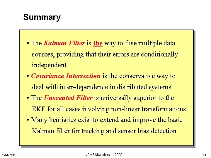
Summary • The Kalman Filter is the way to fuse multiple data sources, providing that their errors are conditionally independent • Covariance Intersection is the conservative way to deal with inter-dependence in distributed systems • The Unscented Filter is universally superior to the EKF for all cases involving non-linear transformations • Many heuristics exist to extend and improve the basic Kalman filter for tracking and sensor bias detection 6 July 2000 NCAF Manchester 2000 24

End of Talk Unless there any questions – make ‘em brief 6 July 2000 NCAF Manchester 2000 25