Gradient Nearest Neighbor Imputation Maps for Landscape Analysis

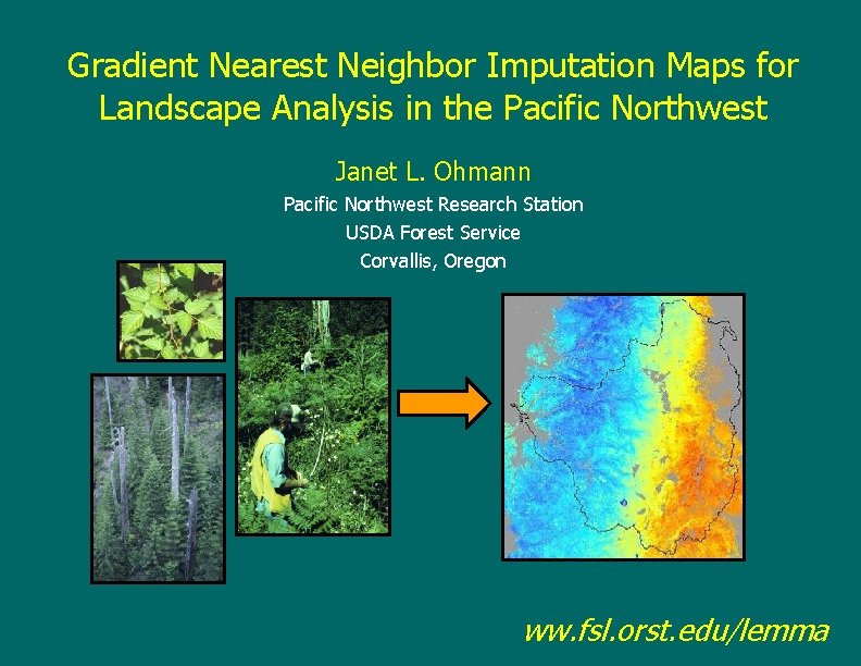
Gradient Nearest Neighbor Imputation Maps for Landscape Analysis in the Pacific Northwest Janet L. Ohmann Pacific Northwest Research Station USDA Forest Service Corvallis, Oregon ww. fsl. orst. edu/lemma

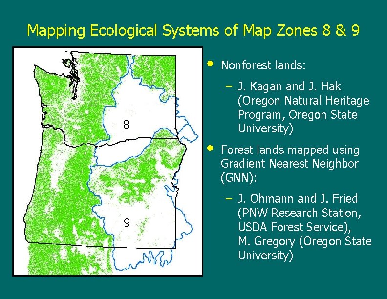
Mapping Ecological Systems of Map Zones 8 & 9 • – J. Kagan and J. Hak (Oregon Natural Heritage Program, Oregon State University) 8 • 9 Nonforest lands: Forest lands mapped using Gradient Nearest Neighbor (GNN): – J. Ohmann and J. Fried (PNW Research Station, USDA Forest Service), M. Gregory (Oregon State University)

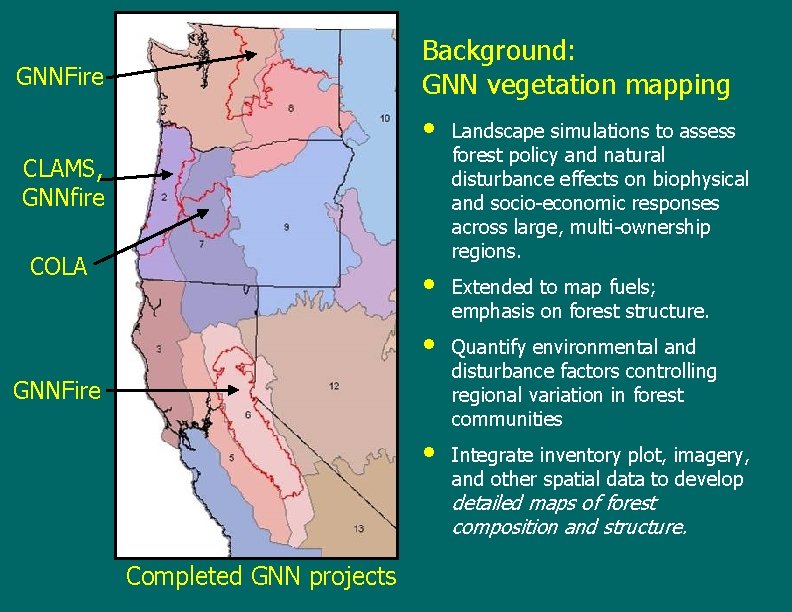
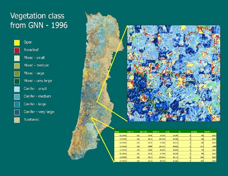
Background: GNN vegetation mapping GNNFire • CLAMS, GNNfire COLA • • GNNFire • Landscape simulations to assess forest policy and natural disturbance effects on biophysical and socio-economic responses across large, multi-ownership regions. Extended to map fuels; emphasis on forest structure. Quantify environmental and disturbance factors controlling regional variation in forest communities Integrate inventory plot, imagery, and other spatial data to develop detailed maps of forest composition and structure. Completed GNN projects

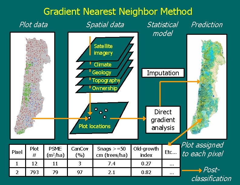
Gradient Nearest Neighbor Method Plot data Spatial data Statistical model Prediction Satellite imagery Climate Geology Topography Ownership Plot locations Imputation Direct gradient analysis Pixel Plot # PSME (m 2/ha) Can. Cov (%) Snags >=50 cm (trees/ha) Old-growth index Etc. . . 1 12 11 3 7. 4 0. 27 . . . 2 793 79 97 2. 1 0. 82 . . . Plot assigned to each pixel Postclassification

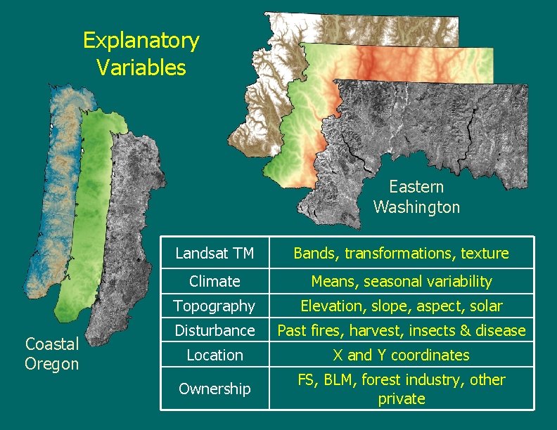
Explanatory Variables Eastern Washington Coastal Oregon Landsat TM Bands, transformations, texture Climate Means, seasonal variability Topography Elevation, slope, aspect, solar Disturbance Past fires, harvest, insects & disease Location X and Y coordinates Ownership FS, BLM, forest industry, other private

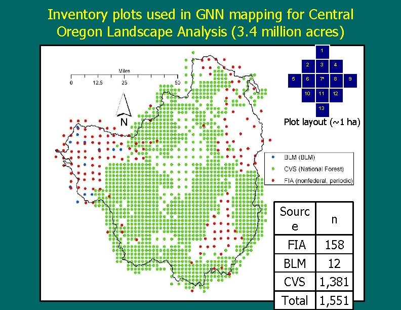
Inventory plots used in GNN mapping for Central Oregon Landscape Analysis (3. 4 million acres) 1 2 3 4 6 7* 8 10 11 12 5 9 13 Plot layout (~1 ha) Sourc e n FIA 158 BLM 12 CVS 1, 381 Total 1, 551

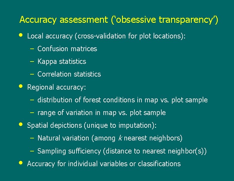
Accuracy assessment (‘obsessive transparency’) • Local accuracy (cross-validation for plot locations): – Confusion matrices – Kappa statistics – Correlation statistics • Regional accuracy: – distribution of forest conditions in map vs. plot sample – range of variation in map vs. plot sample • Spatial depictions (unique to imputation): – Natural variation (among k nearest neighbors) – Sampling sufficiency (distance to nearest neighbor(s)) • Accuracy for individual variables or classifications

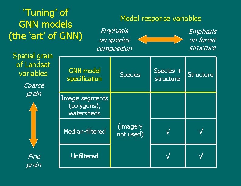
‘Tuning’ of GNN models (the ‘art’ of GNN) Spatial grain of Landsat variables Coarse grain Model response variables Emphasis on species composition GNN model specification Species + Structure structure Image segments (polygons), watersheds Median-filtered Fine grain Species Emphasis on forest structure Unfiltered (imagery not used) √ √

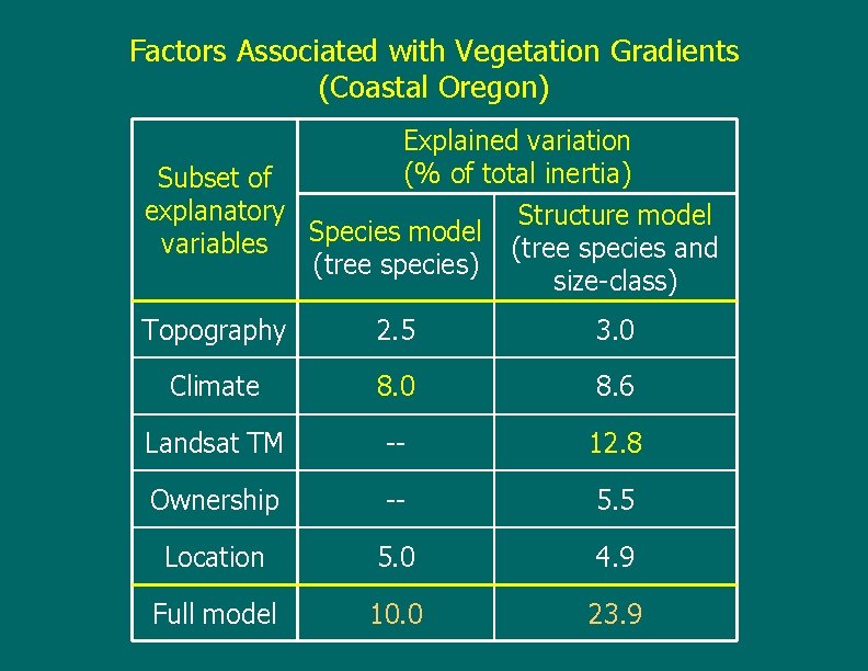
Factors Associated with Vegetation Gradients (Coastal Oregon) Explained variation (% of total inertia) Subset of explanatory Species model variables (tree species) Structure model (tree species and size-class) Topography 2. 5 3. 0 Climate 8. 0 8. 6 Landsat TM -- 12. 8 Ownership -- 5. 5 Location 5. 0 4. 9 Full model 10. 0 23. 9

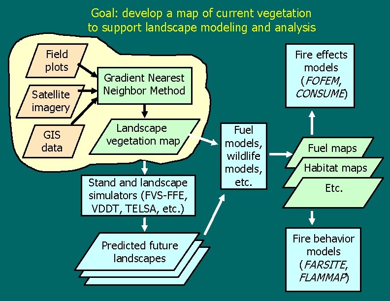
Goal: develop a map of current vegetation to support landscape modeling and analysis Field plots Satellite imagery GIS data Fire effects models (FOFEM, CONSUME) Gradient Nearest Neighbor Method Landscape vegetation map Stand landscape simulators (FVS-FFE, VDDT, TELSA, etc. ) Predicted future landscapes Fuel models, wildlife models, etc. Fuel maps Habitat maps Etc. Fire behavior models (FARSITE, FLAMMAP)

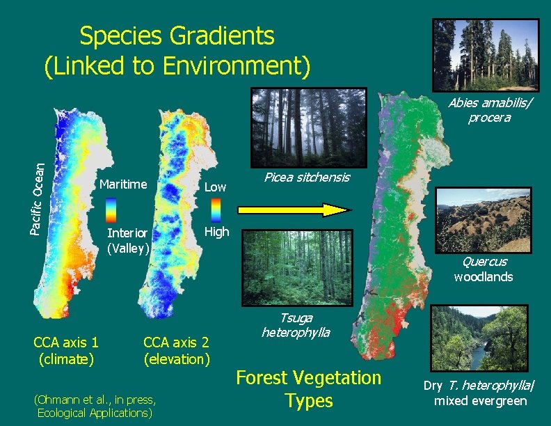
Species Gradients (Linked to Environment) Pacific Ocean Abies amabilis/ procera Maritime Low Interior (Valley) High Picea sitchensis Quercus woodlands CCA axis 1 (climate) CCA axis 2 (elevation) (Ohmann et al. , in press, Ecological Applications) Tsuga heterophylla Forest Vegetation Types Dry T. heterophylla/ mixed evergreen

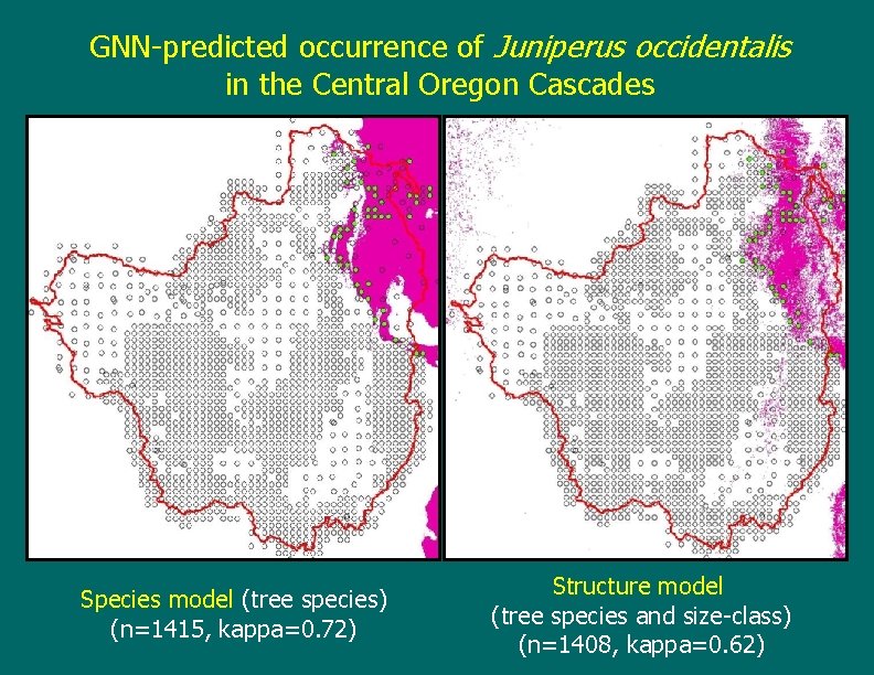
GNN-predicted occurrence of Juniperus occidentalis in the Central Oregon Cascades Species model (tree species) (n=1415, kappa=0. 72) Structure model (tree species and size-class) (n=1408, kappa=0. 62)

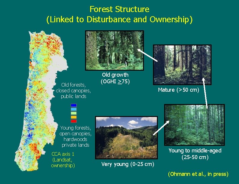
Forest Structure (Linked to Disturbance and Ownership) Old forests, closed canopies, public lands Old growth (OGHI >75) Mature (>50 cm) Young forests, open canopies, hardwoods private lands CCA axis 1 (Landsat, ownership) Young to middle-aged (25 -50 cm) Very young (0 -25 cm) (Ohmann et al. , in press)

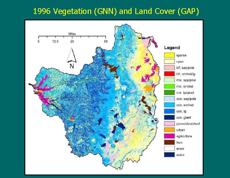
1996 Vegetation (GNN) and Land Cover (GAP)

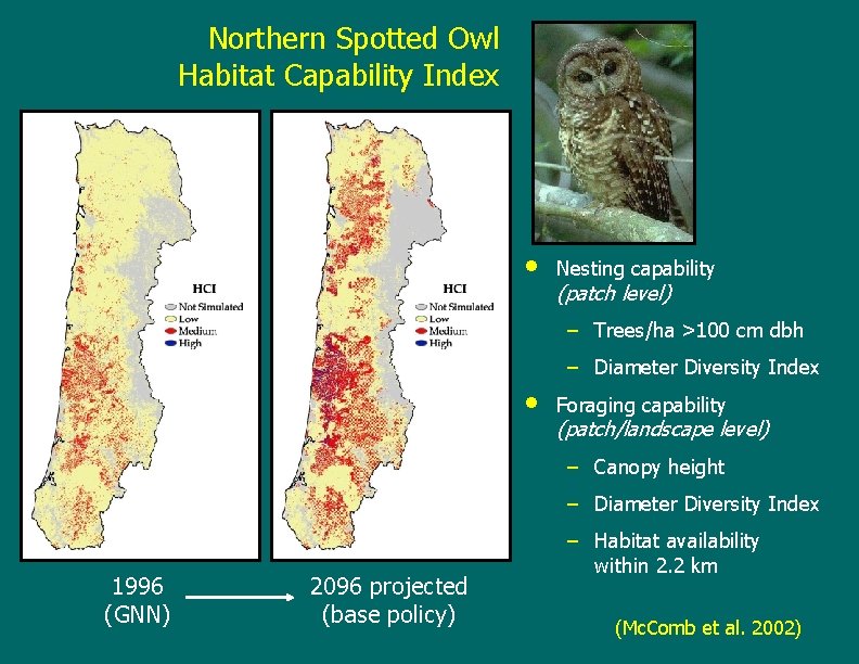
Northern Spotted Owl Habitat Capability Index • Nesting capability (patch level) – Trees/ha >100 cm dbh – Diameter Diversity Index • Foraging capability (patch/landscape level) – Canopy height – Diameter Diversity Index 1996 (GNN) 2096 projected (base policy) – Habitat availability within 2. 2 km (Mc. Comb et al. 2002)

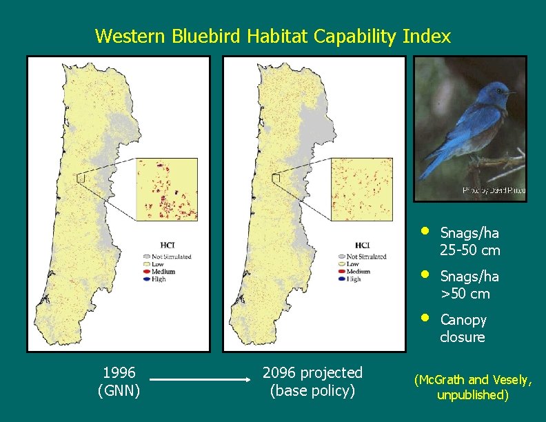
Western Bluebird Habitat Capability Index • • • 1996 (GNN) 2096 projected (base policy) Snags/ha 25 -50 cm Snags/ha >50 cm Canopy closure (Mc. Grath and Vesely, unpublished)

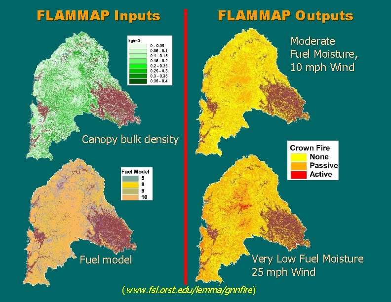
FLAMMAP Inputs FLAMMAP Outputs Moderate Fuel Moisture, 10 mph Wind Canopy bulk density Fuel model Very Low Fuel Moisture 25 mph Wind (www. fsl. orst. edu/lemma/gnnfire)

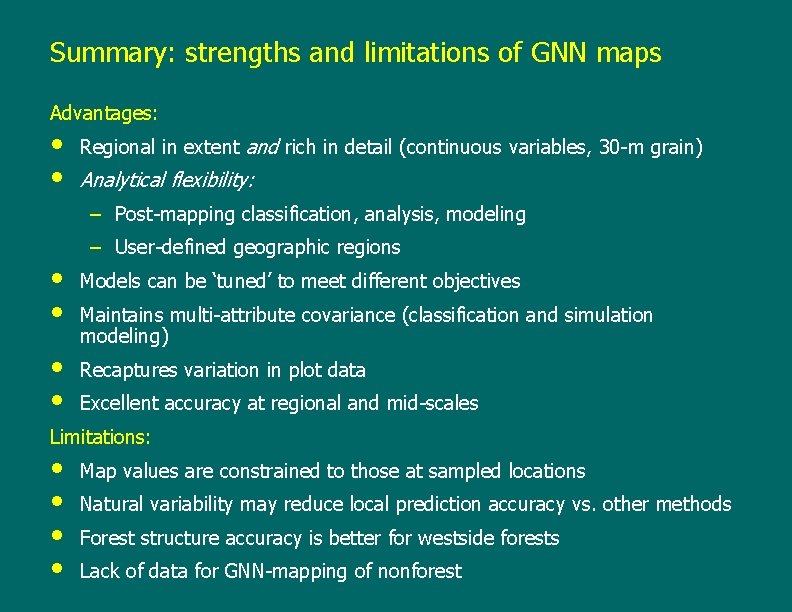
Summary: strengths and limitations of GNN maps Advantages: • • Regional in extent and rich in detail (continuous variables, 30 -m grain) Analytical flexibility: – Post-mapping classification, analysis, modeling • • – User-defined geographic regions Models can be ‘tuned’ to meet different objectives Maintains multi-attribute covariance (classification and simulation modeling) Recaptures variation in plot data Excellent accuracy at regional and mid-scales Limitations: • • Map values are constrained to those at sampled locations Natural variability may reduce local prediction accuracy vs. other methods Forest structure accuracy is better for westside forests Lack of data for GNN-mapping of nonforest