Gradient Nearest Neighbor GNN Method for LocalScale Basal
Gradient Nearest Neighbor (GNN) Method for Local-Scale Basal Area Mapping: FIA 2005 Symposium Interpolation Contest Kenneth B. Pierce Jr. , Matthew J. Gregory* and Janet L. Ohmann Forestry Science Lab, 3200 SW Jefferson Way, Corvallis OR 97331
Why map? Why GNN? (Pacific Northwest perspective) • • Primary objective: supply missing data for analysis and modeling of forest ecosystems at the regional level Problem: basic information on current vegetation is needed to address a wide array of issues in forest management and policy. Increasingly, this information needs to be: – spatially complete (spatial pattern, small geographic areas) – consistent across large, multi-ownership regions – rich in floristic and structural detail – suitable for input to stand landscape simulation models • – flexible in meeting a variety of analytical needs Differs from other objectives which are concerned primarily with estimation
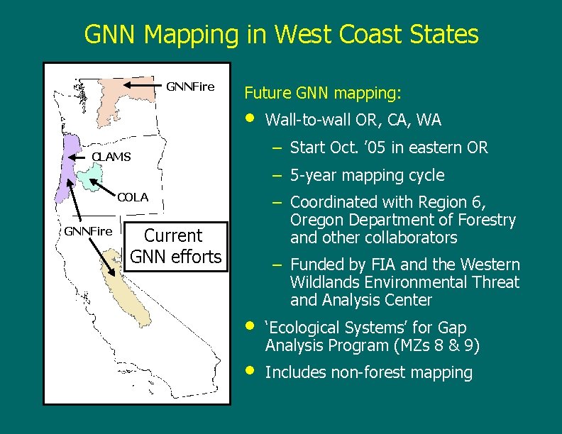
GNN Mapping in West Coast States GNNFire Future GNN mapping: • Wall-to-wall OR, CA, WA – Start Oct. ’ 05 in eastern OR CLAMS – 5 -year mapping cycle COLA GNNFire – Coordinated with Region 6, Oregon Department of Forestry and other collaborators Current GNN efforts • • – Funded by FIA and the Western Wildlands Environmental Threat and Analysis Center ‘Ecological Systems’ for Gap Analysis Program (MZs 8 & 9) Includes non-forest mapping
The Gradient Nearest Neighbor (GNN) Method for Vegetation Mapping • A tool for: – Spatially explicit (wall-to-wall) vegetation data based on ‘interpolation’ of FIA plot data using an ecological (gradient) model – Inference of plot data to smaller geographic areas (e. g. , 6 th-field HUCs) • Imputation approach (as are k. NN, MSN) provides: – Data that are regional in extent, yet rich in detail – Analytical flexibility for users
• Components of GNN Imputation Statistical model = canonical correspondence analysis (CCA) (flexibility for redundancy analysis (RDA) and other methods): – Multivariate – Results in a weight for each of many spatial variables, based on its relationship with the multiple response variables • – Any multivariate method can be specified (eg. PCA, CCor. A) Distance measure (between map pixel and potential NN plots): – Euclidean distance for first n axes (usually 8, specified by user) • – Axes weighted by their explanatory power (eigenvalues) Imputation method: – Single nearest neighbor (k=1, MSN-like) – Summary statistic of multiple neighbors (k. NN-like) – Measures of variation based on multiple imputation (k>1)
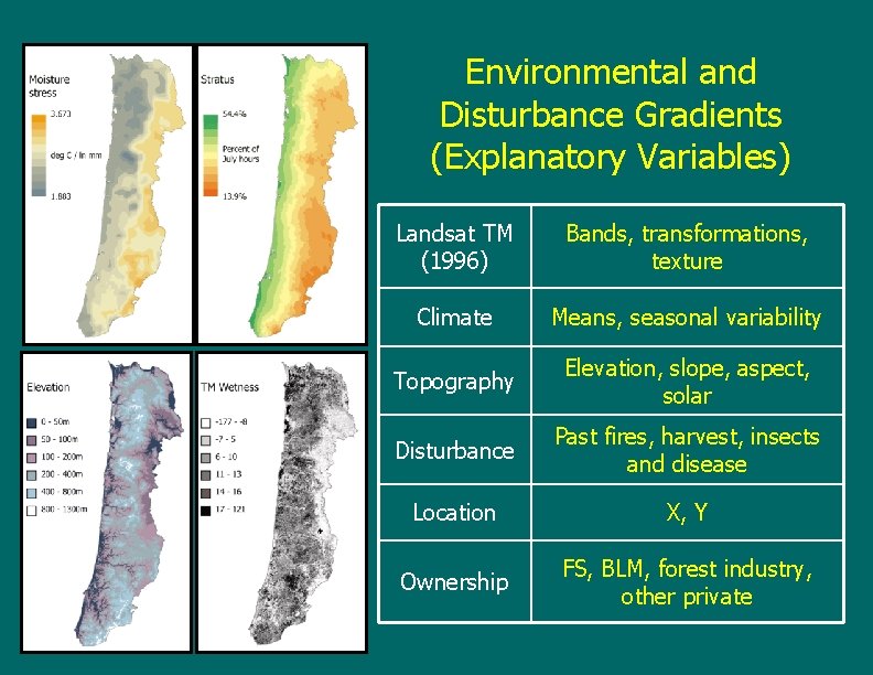
Environmental and Disturbance Gradients (Explanatory Variables) Landsat TM (1996) Bands, transformations, texture Climate Means, seasonal variability Topography Elevation, slope, aspect, solar Disturbance Past fires, harvest, insects and disease Location X, Y Ownership FS, BLM, forest industry, other private
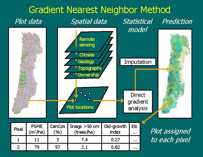
Gradient Nearest Neighbor Method Plot data Spatial data Statistical model Prediction Remote sensing Climate Geology Topography Ownership Imputation Direct gradient analysis Plot locations Pixel PSME (m 2/ha) Can. Cov Snags >50 cm (%) (trees/ha) 1 11 3 2 79 97 Old-growth index Etc. . . 7. 4 0. 27 . . . 2. 1 0. 82 . . . Plot assigned to each pixel
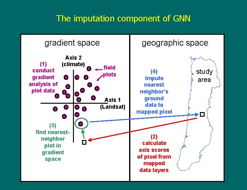
The imputation component of GNN gradient space (1) conduct gradient analysis of plot data Axis 2 (climate) geographic space field plots Axis 1 (Landsat) (3) find nearestneighbor plot in gradient space (4) impute nearest neighbor’s ground data to mapped pixel (2) calculate axis scores of pixel from mapped data layers study area
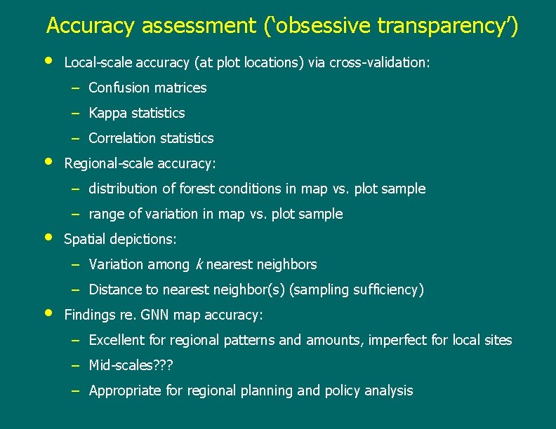
Accuracy assessment (‘obsessive transparency’) • Local-scale accuracy (at plot locations) via cross-validation: – Confusion matrices – Kappa statistics – Correlation statistics • Regional-scale accuracy: – distribution of forest conditions in map vs. plot sample – range of variation in map vs. plot sample • Spatial depictions: – Variation among k nearest neighbors – Distance to nearest neighbor(s) (sampling sufficiency) • Findings re. GNN map accuracy: – Excellent for regional patterns and amounts, imperfect for local sites – Mid-scales? ? ? – Appropriate for regional planning and policy analysis
Bartlett Interpolation Contest • • Comparison between ‘control’ methods and GNN methods Effect of footprint size
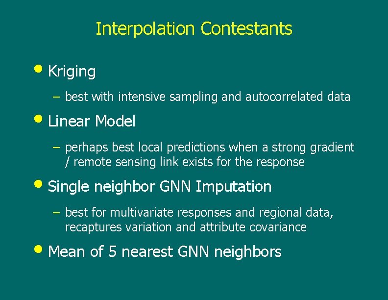
Interpolation Contestants • Kriging – best with intensive sampling and autocorrelated data • Linear Model – perhaps best local predictions when a strong gradient / remote sensing link exists for the response • Single neighbor GNN Imputation – best for multivariate responses and regional data, recaptures variation and attribute covariance • Mean of 5 nearest GNN neighbors
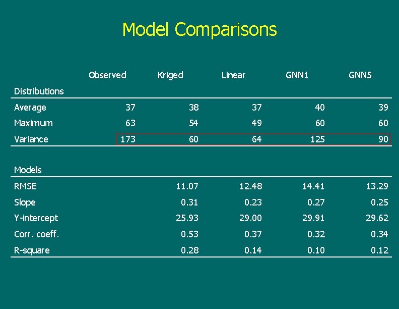
Model Comparisons Observed Kriged Linear GNN 1 GNN 5 Distributions Average 37 38 37 40 39 Maximum 63 54 49 60 60 Variance 173 60 64 125 90 RMSE 11. 07 12. 48 14. 41 13. 29 Slope 0. 31 0. 23 0. 27 0. 25 Y-intercept 25. 93 29. 00 29. 91 29. 62 Corr. coeff. 0. 53 0. 37 0. 32 0. 34 R-square 0. 28 0. 14 0. 10 0. 12 Models
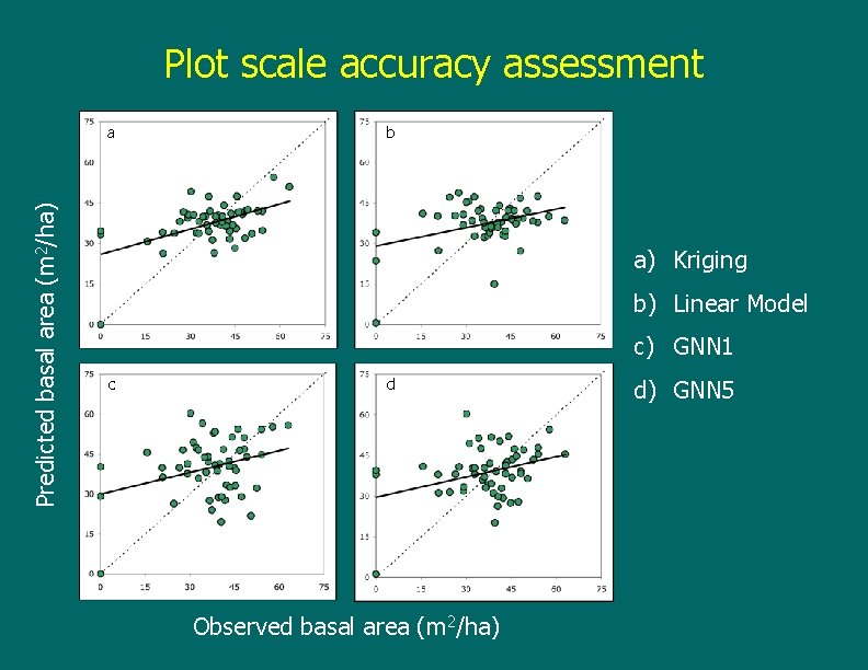
Plot scale accuracy assessment Predicted basal area (m 2/ha) a b a) Kriging b) Linear Model c) GNN 1 c d Observed basal area (m 2/ha) d) GNN 5
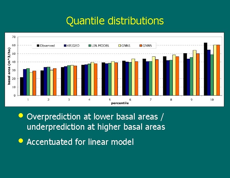
Quantile distributions • Overprediction at lower basal areas / underprediction at higher basal areas • Accentuated for linear model
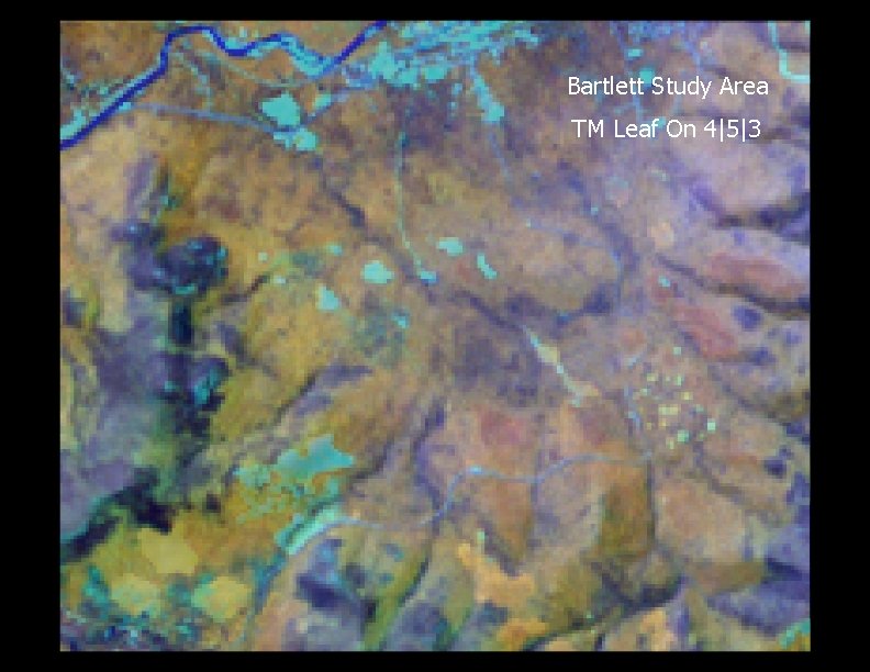
Bartlett Study Area TM Leaf On 4|5|3
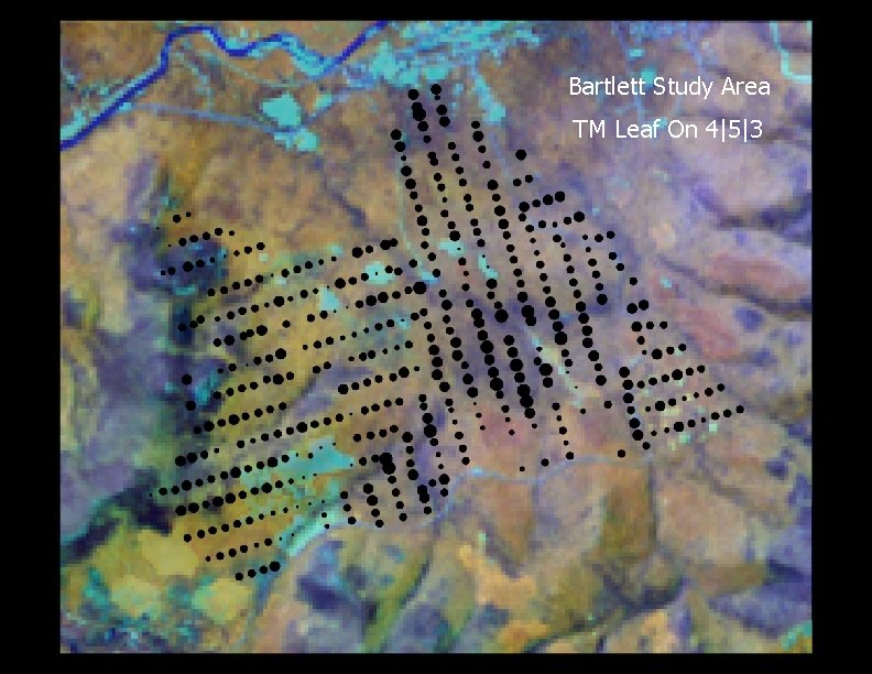
Bartlett Study Area TM Leaf On 4|5|3
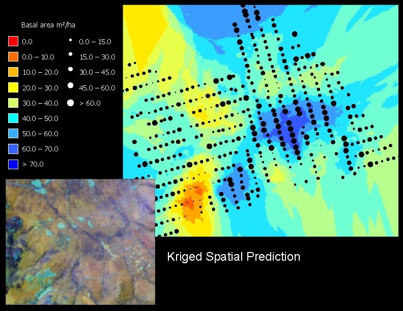
Basal area m 2/ha 0. 0 – 15. 0 0. 0 – 10. 0 15. 0 – 30. 0 10. 0 – 20. 0 30. 0 – 45. 0 20. 0 – 30. 0 45. 0 – 60. 0 30. 0 – 40. 0 > 60. 0 40. 0 – 50. 0 – 60. 0 – 70. 0 > 70. 0 Kriged Spatial Prediction
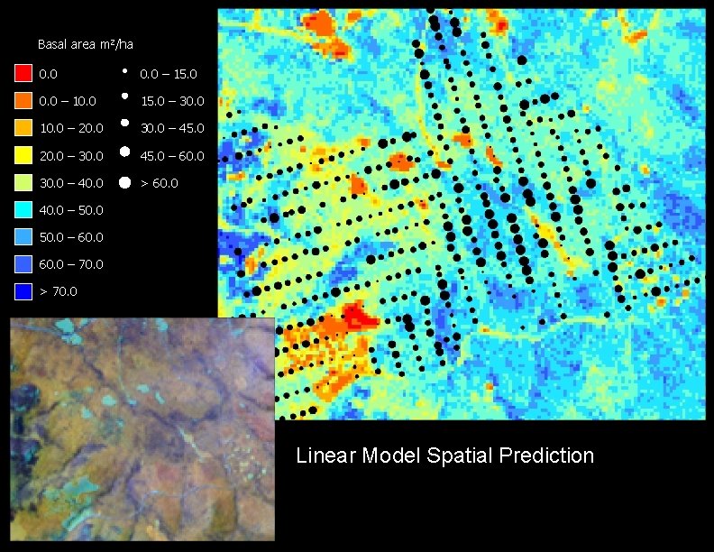
Basal area m 2/ha 0. 0 – 15. 0 0. 0 – 10. 0 15. 0 – 30. 0 10. 0 – 20. 0 30. 0 – 45. 0 20. 0 – 30. 0 45. 0 – 60. 0 30. 0 – 40. 0 > 60. 0 40. 0 – 50. 0 – 60. 0 – 70. 0 > 70. 0 Linear Model Spatial Prediction
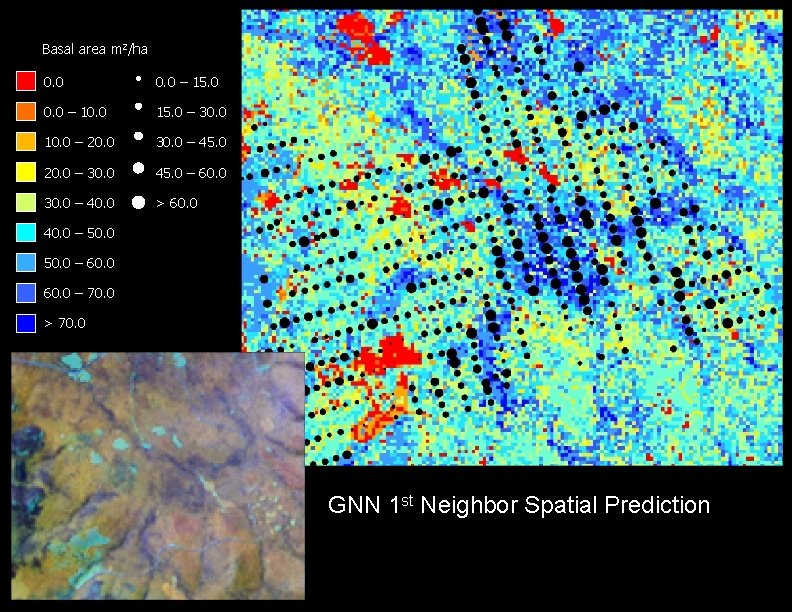
Basal area m 2/ha 0. 0 – 15. 0 0. 0 – 10. 0 15. 0 – 30. 0 10. 0 – 20. 0 30. 0 – 45. 0 20. 0 – 30. 0 45. 0 – 60. 0 30. 0 – 40. 0 > 60. 0 40. 0 – 50. 0 – 60. 0 – 70. 0 > 70. 0 GNN 1 st Neighbor Spatial Prediction
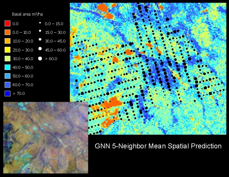
Basal area m 2/ha 0. 0 – 15. 0 0. 0 – 10. 0 15. 0 – 30. 0 10. 0 – 20. 0 30. 0 – 45. 0 20. 0 – 30. 0 45. 0 – 60. 0 30. 0 – 40. 0 > 60. 0 40. 0 – 50. 0 – 60. 0 – 70. 0 > 70. 0 GNN 5 -Neighbor Mean Spatial Prediction
Effect of plot footprint size • • Studied to account for possible misregistration between plots and TM imagery Used two footprints at 30 m cell resolution – 1 x 1 and 2 x 2 (plot spacing is ~65 m – 3 x 3 windows overlap) – Used for both extraction of spatial data and for mean basal area prediction at the cross-validation plots • Imputation is still at a per-pixel level
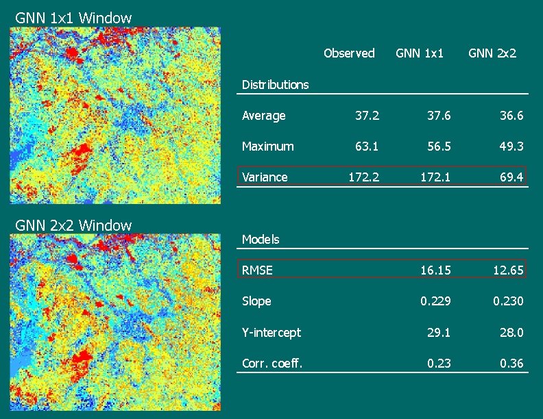
GNN 1 x 1 Window Observed GNN 1 x 1 GNN 2 x 2 Distributions GNN 2 x 2 Window Average 37. 2 37. 6 36. 6 Maximum 63. 1 56. 5 49. 3 Variance 172. 2 172. 1 69. 4 RMSE 16. 15 12. 65 Slope 0. 229 0. 230 Y-intercept 29. 1 28. 0 Corr. coeff. 0. 23 0. 36 Models
Summary – Bartlett Interpolation • • Inverse relationship between better model fits and maintaining sample variance between methods While kriging gives the highest degree of local scale agreement, it suffers from lack of spatial pattern Linear model and GNN imputation methods seem to maintain spatial pattern Plot footprint size made larger difference than anticipated
Strengths and limitations of GNN imputation Advantages: • Recaptures most of variation in plot data • Maintains multi-attribute covariance at a location • Analytical flexibility: detailed vegetation data for postmapping classification, analysis, and modeling • Ability to map variability and assess sampling sufficiency • Where strong gradients exist, can use other spatial environmental data to describe pattern Limitations: • Map values are constrained to those at sampled locations • Natural variability reduces local-scale prediction accuracy
- Slides: 24