Gradient echo sequences and SWI Dr Harish K

Gradient echo sequences and SWI Dr Harish K Gowda

MR SIGNAL

MR SEQUENCE • Carefully co-ordinated and timed series of events to generate particular type of image contrast.

Classification • Spine Echo sequence – Echoes are rephased by 1800 rephasing pulse • Gradient sequence – Echoes are rephased by gradients

Various types of sequences Spin Echo Seq. Conventional spin E. Fast or turbo spin E. Inversion recovery. Gradient Echo Seq Coherent gradient E. Incoherent gradient E. SSFP Balanced gradient E. Fast gradient E. EPI

What is T 2* Relaxation? T 2* Relaxation is combination of true T 2 relaxation and magnetic field inhomogenities

T 2* Relaxation • Main magnetic field inhomogeneity, • the differences in magnetic susceptibility among various tissues or materials, • chemical shift, • and gradients applied for spatial encoding

Comparison of SE and GRE Sequences Criterion SE GRE Rephasing mechanism RF pulse Variation of gradients Flip angle 90° only Variable Efficiency at Very efficient reducing (true T 2 magnetic weighting) inhomogeneity Not very efficient (T 2* weighting)

GRADIENT ECHO SEQUENCES

GRE sequences can be T 1 W Large flip angle (70 -110) Short TR <50 ms Short TE 5 -10 ms T 2 W small flip angle (5 -20) Long TR Long TE 15 -25 ms

PD W • Small flip angle (5 -20) • Long TR • Short TE 5 -10 ms

THE STEADY STATE Ø State where TR is shorter than T 1 and T 2 relaxation time of the tissue. Ø To achieve this, energy given to H 2 atom should be equal to energy lost by H 2 atom. Ø Flip angle of 30 -45⁰ and TR – 20 -50 ms Ø In SS image contrast is not due to differences in T 1 and T 2 relaxation times of tissues but due to ratio of T 1 and T 2.

STEADY STATE

THE STEADY STATE AND ECHO FORMATION Ø GE sequences can be classified accn to residual transverse magnetization as Ø - Coherent ( tr. Magnetization in phase ) Ø - Incoherent ( tr. Magenetiazation out of phase)

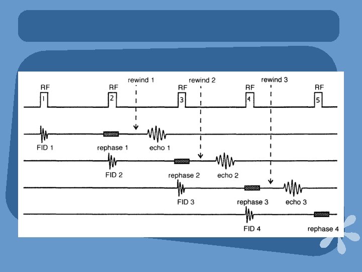
ECHO FORMATION IN SS Ø In SS , repeated RF pulses applied at an time interval less than T 1 and T 2 relaxation time of all tissues, producing 2 signals: Ø * A FID signal : occurs as a result of withdrawal of the RF pulse and contains T 2* and T 1 info. Ø * A Spin echo : occurs at the same time of next RF pulse. Ø Contains T 2* and T 2 info.

ECHO FORMATION IN SS

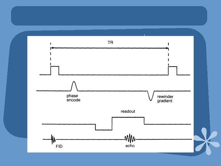
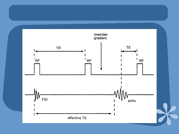
COHERENT GRADIENT ECHO Ø GRASS ( GE ) , FFE ( PHILIPS ), FISP ( SIEMENS) Ø Use variable flip angle excitation pulse followed by rephasing gradient to produce gradient echo. Ø Residual transevese magnetization is kept coherent by rewinding.

Ø Rewinding is achieved by reversing the slope of phase encoding gradient after readout. Ø The rewinder gradient rephases all transverse magnetization hence it contain info from both FID and stimulated echoes. Ø Used to produce T 2 W images

Ø Adv: Ø 1. Very fast scans, hence breath holding is possible. Ø 2. Very sensitive to flow – Angiography. Ø 3. Myelography , arthrography. Ø 4. Can be acquired in volume acquisition. Ø Disadv: Ø 1. Poor SNR in 2 D acquisitions. Ø 2. Increased magenetic susceptibilty.

PARAMETERS Ø To maintain SS: Ø Flip angle : 30 -45⁰ Ø TR : 20 -50 ms Ø To maximize T 2*: Ø Long TE - 15 -25 ms Ø GMR can be used to accentute T 2* and to reduce flow artefacts. Ø Avg Scan time : Sec for single slice , 4 -15 min for vol.

INCOHERENT GRADIENT ECHO Ø SPGR /MPGR(GE), T 1 FFE (Philips ), FLASH ( Siemens) Ø Similar to coherent gradient echo except that the residual tr. Mag is dephased so that its effect on image contrast is minimal. Ø Tr. Mag from previous excitation is used only hence predominantly T 1 W image. Ø Dephasing is done by either RF spoiling or Gradient spoiling.

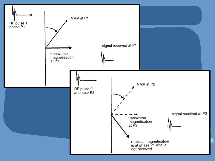
Digitized RF Spoiling(SPGR) • RF is transmitted at a particular frequency to excite a slice and at a specific phase. • The receiver coil digitally communicates with the transmit coil and only frequencies from echo that just has been created are digitized. • Tr. Mag in another phase or position is not received by receiver coil.

Gradient Spoiling (MPGR) Ø Opposite of rewinding. Ø The slice select, phase encoding and frequency encoding gradients are used to dephase the residual magnetization. Ø Hence it is incoherent at the beginning of next repetition.

Uses of SPGR Ø SPGR sequences produce T 1 or PDW images. Ø Can be used 2 D or vol. acquisition. Ø As TR is short can be used for T 1 W breath holding sequences. Ø Demonstrate good T 1 W anatomy.

3 D SPGR

Parameters of SPGR Ø To maintain steady state : Flip angle – 30 -45⁰ TR - 20 - 50 ms Ø To maximize T 1 : Short TE : 5 -10 ms Avg scan time : several sec for single slice 4 -15 min for volume

Ø Adv: * Can be acquired in vol or 2 D. * Breath holding is possible. * Good SNR and anatomical details. Ø Disadv: * SNR poor in 2 D. * Loud gradient noise.

STEADY STATE FREE PRECESSION Ø SSFP( GE), T 2 FFE (PHILIPS), PSIF( SIEMENS) Ø In Gr. Echo sequences TE is not enough ( atleast 70 ms) for true T 2 w imaging. Ø SSFP provides sufficiently long TE and less T 2* Ø In SSFP, only frequncies from stimulated echoes are digitized and not from FIDs.

STEADY STATE FREE PRECESSION Ø It is achieved by applying rewinder gradient which speeds up the rephasing process initiated by RF pulse. Hence stimulated echo occurs just before the next excitation pulse.

Ø Resultant echo is more T 2 W and contain 2 TEs. - Actual TE – time betn echo and next excitaion pulse. - Effective TE – time from echo to the excitation pulse that created its FID. Effective TE = (2 x. TR ) - TE

Parameters of SSFP • To maintain steady state: Flip angle – 30 -45⁰ TR - 20 - 50 ms • Actual TE affect the effective TE. More the actual TE less the effective TE. • Avg scan time : 4 -15 min.

USES of SSFP Ø ADV: • To demonstrate true T 2 weighing. • Esp in brain and joint imaging. • Can be used in both 2 D and 3 D acquisition. Ø Disadv: • Susceptible for artefacts. • Poor image quality.

GRASS/FFE/FISP (CGRE)

SPGR/T 1 FFE/FLASH(IGRE)

SSFP/T 2 FFE/PSIF

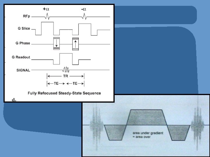
BALANCED GRADIENT ECHO • FIESTA (GE), BFFE (PHILIPS), TRUE FISP(SIEMENS), CISS • Modification of coherent gradient echo. • T 2 W 3 D sequence. • Uses balanced gradient system to correct for phase errors in flowing blood and CSF and alternating RF excitation to enhance steady state.

PARAMETERS OF BGRE • Balanced frequency readout gradient. • Higher flip angles and shorter TR to maintain steady state. • Complete TR is not applied in single TR but it is applied in succesive TR with alternative polarity.

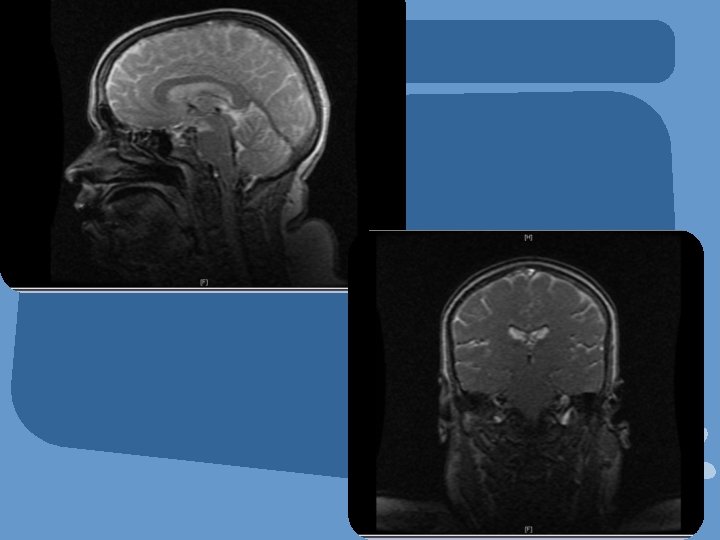
Uses Of FIESTA Ø 3 D acuqisition of posterior cranial fossa gives high resolution images showing cranial nerves dark against background of bright CSF. Ø Esp used for suspected IAC and CP angle pathologies. Ø Also used to visualise spinal nerve roots and optic nerve.

AX 2 D FIESTA

ULTRA FAST SEQUENCES Ø Fast gradient echo (FGRE) Ø Echo planar imaging (EPI) SE- EPI GE-EPI

FAST GRADIENT ECHO Ø Fast gradient echo (FGRE) sequences (also known as turbo GE or ultrafast GE sequences) used in conjunction with state-of-the-art gradient systems (active shielding) achieve TE below 1 ms with TR of 5 ms or less. Ø Fast GRE is basically a conventional GRE sequence that is run faster imaging only part of RF pulse is applied and only part of echo is read. . )

FAST GRADIENT ECHO Ø Fast GRE - yield an excellent image quality although a slice can be acquired in only a few seconds (typically 2– 3 sec). Ø Highly suitable for dynamic imaging, for example, to track the inflow of a contrast medium bolus. Ø For imaging body regions where motion artifacts must be eliminated such as the chest (respiratory motion) and the abdomen (peristalsis).

K-SPACE FILLING IN FGRE Ø CENTRIC K SPACE FILLING -Central k spaces are filled first. -signal and contrast are maximized as central k spaces are filled when echoes have their highest amplitude. Ø KEYHOLE K SPACE FILLING: - K spaces are filled linearly except central k spaces are filled during specific part of seq. - Used in CEMRA.

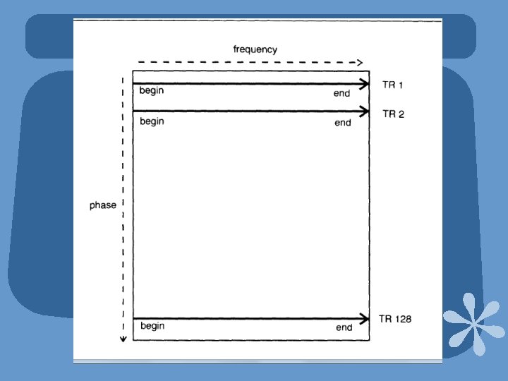
ECHO PLANAR IMAGING(EPI) Ø Echo planar imaging (EPI) enables ultrafast data acquisition, making it an excellent candidate for dynamic and functional MR imaging. Ø Term given by Sir Peter Mansfield in 1977. Ø This method requires strong and rapidly switched frequency and phase encoding gradients. Ø A single echo train is used to fill all the lines of k space.

ECHO PLANAR IMAGING(EPI) Ø To fill all K spaces in single TR readout and phase encode gradients must rapidly switch on and off and change their polarity. Ø There are different ways of filling k space in EPI. 1. Oscillation of frequency , blipping of phase. 2. Spiral K space filling.

Oscillation of frequency , blipping of phase

Spiral k space filling

PARAMETERS FOR EPI Ø PD or T 2 W images can be obtained by selecting short or long effective TE. Ø EPI can be done with spin echo (SE-EPI) or gradient echo (GE-EPI). Ø Hybrid Sequence which combine gradient and spin echo( GRASE). Ø Benifit of both types of rephasing Ø Speed of gradient rephasing and T 2* compensation of spin echo rephasing.

SWI

Susceptibility Weighted Imaging • Idea of phase imaging as new contrast enhancing parameter. • Phase imaging contains information of susceptibility differences between the different tissues. • Only magnitude imaging was used clinically till now. • Other contrast parameters T 1 recovery and T 2* decay, TR NEX.

Applications of SWI • SWI offers information about tissues with different susceptibilities from surrounding tissues. – deoxygenated blood, hemosiderin, ferritin, calcium • Numerous Clinical applications – – – Hemorrhages Cerebrovascular and ischemic brain diseases Traumatic brain injuries Arteriovenous malformations Neurodegenerative diseases Breast microcalcifications

Currently • Packaged SWI technique available on Siemens Medical Systems. • SWAN on GE scanner: T 2 Star Weighted Angiography. (multi-echo GRE) uses echoes.

Magnetic Susceptibility • When an object is placed in an external magnetic field H, magnetization is induced in the object. • Magnetic susceptibility is the magnetic response of a material when it is placed in a magnetic field. – M = χH – χ = susceptibility (ppm) – M = induced magnetization – H = applied field • If diamagnetic, like Ca 3(PO)4, χ < 0 • If paramagnetic, like deoxygenated blood, χ > 0 E. M. Haacke et. Al. Susceptibility-Weighted Imaging: Technical Aspects and Clinical Applications, 64 Part 1. AJNR Am J Neuroradiol 30: 19 -30. Jan 2009.

Susceptibility and Phase Relations • MRI equations – ω=γB 0 larmor equation – ψ=ωt phase equation – Δψ=Δω*TE • Relating to susceptibility, – Since Δω=γΔB and ΔB=g*Δχ*B 0 – Δψ=-γΔB*TE – And so, Δψ=-γgΔχB 0*TE 65

Effect of sample shape, orientation and susceptibility Schenck, JF. The role of magnetic susceptibility in magnetic resonance imaging: MRI magnetic 66 compatibility of the first and second kinds. Med Phys. 1996 Jun; 23(6): 815 -50

Outline of SWI Processing 1. Acquire high-res 3 D f. GRE. 2. Apply HPF to phase image to obtain “SWI filtered phase data. ” 3. Create “phase” mask. 4. Multiply phase mask by original magnitude image to obtain “merged SWI magnitude data. ” 67

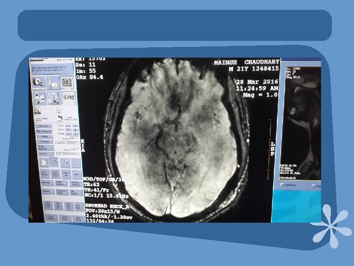
Step 1: Acquisition Magnitude 68 c/o Samantha Holdsworth

Step 2: Creating HPF • Uses 64 x 64 low-pass filter divided into the original phase image to create a HP -filter effect. • Method 1. Truncate original image ρ(r) to central n x n complex image ρn(r). 2. Zero-fill elements outside central n x n elements 3. Complex divide ρ(r) by ρn(r) to obtain a new image, ρ’(r) = ρ(r)/ρn(r) 69

Step 2: Phase Images Raw phase image HP-filtered (32 x 32) HP-filtered (64 x 64) Fig. 3 Haacke Review 1 70

Step 3: Phase Mask • Intratissue phase and extratissue phase which impair the differentiation of adjacent tissues with different susceptibility • Phase mask between 0 to 1 E. M. Haacke et. al. Susceptibility Weighted Imaging. MRM 52: 612 -618 (2004). 71

Step 3: Phase Masking Process Phase profile in filtered phase image Fig. 6 Haacke Review 1 Profile of mask created from A 72

Step 4: Simulated images with phase mask multiplication ρ(x)new= fm(x)ρ(x) m=1 m=4 m=8 m=16 The smaller the phase value, the larger the multiplication required to reach the maximum CNR Fig. 1 Haacke 73

Overview: SWI Processing Magnitude image (phase mask)m SWI image SWI min. IP X Phase image ≥ 4 images 74 c/o Samantha Holdsworth

IMAGE INTERPRETATION • Greyscale inversion filtered phase images are not uniformly windowed or presented equally by all manufacturers, therefore care must be taken to ensure correct interpretation. • A simple step to make sure that you always view the images in the same way is to look at venous structures & compare them with the lesions. The lesions with blood or ferritin (paramagnetic) will have the same signal as veins. Mittal. S et al. Susceptibility-Weighted Imaging: Technical Aspects and Clinical Applications. AJNR 2009

IMAGE INTERPRETATION Magnitude Phase CT Note that calcifications on the phase (center) image have different signal than blood in the sagittal sinus (arrow). Mittal. S et al. Susceptibility-Weighted Imaging: Technical Aspects and Clinical Applications. AJNR 2009

CLINICAL APPLICATIONS

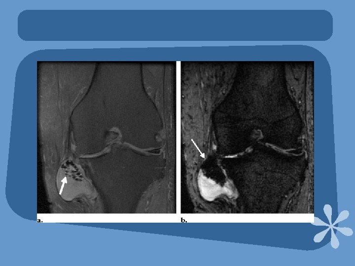
DIFFERENTIATION BETWEEN MICROBLEED FROM MICROCALCIFICATIONS • Both calcifications & iron accumulation in chronic hemorrhage are hypointense on T 2 -WI & show “blooming” in SWI. It is not possible to differentiate between them on conventional MR sequences & CT is usually required. • SWI - phase represents an average magnetic field of protons in a voxel, which depends on the susceptibility of tissues. • Calcium is diamagnetic in nature and the phase shift induced by it is opposite to that found with paramagnetic substances like deoxy-Hb, methemoglobin (Met-Hb), hemosiderin & ferritin. Yamada et al. Intracranial calcification on gradient-echo phase image: depiction of diamagnetic susceptibility. Radiology. 1996

DIFFERENTIATION BETWEEN MICROBLEEDS AND MICROCALCIFICATIONS - AMYLOID ANGIOPATHY A B. SWI (A) shows subcortical black spots in parietal/occipital regions. One cannot be sure if they correspond to microhemorrhages or calcifications. In SWI-Phase (B) the spots have similar signal to that of the deep venous structures (black arrow) indicating that they correspond to blood.

DIFFERENTIATION BETWEEN MICROBLEEDS AND MICROCALCIFICATIONS - POST-RADIOTERAPHY A B High grade glioma after radiotherapy. SWI (A) cannot differentiate if the signal loss in the ventricular system & occipital lobes are due to choroid plexus microcalcifications or microhemorrhages. SWI-Phase (B) shows bright spots similar in signal to blood in the deep venous system (arrow) suggesting microhemorrhages instead of calcifications.

SWI in Multiple Sclerosis MS Patient Normal Volunteer Iron build up in the pulvinar in MS indicated with SWI 81 Haacke Review, Part 2

Sturge Weber Syndrome in 5 y. o. girl Post-contrast T 1 w Leptomeninges (arrowhead) Periventricular veins (arrow) SWI – calcification of gyri (dotted/arrowhead) Periventricular veins (arrow) Sturge-Weber Syndrome found most often in children leads to vascular 82 malformation Haacke Review, Part 2

Occult Venous angioma

DAI

Stroke and Hemorrhage

TUMOR CHARACTERIZATION • Many imaging characteristics have been suggested to predict glioma grade including heterogeneity, contrast enhancement, mass effect, necrosis, metabolic activity & high cerebral blood volume. In human glioma cells, levels of ferritin & transferrin receptors detected during immunohistochemical analysis correlate with tumor grade. • SWI-Phase helps to detect calcifications and/or blood, therefore, improving accuracy in interpretation of brain tumors & aiding in grading. Thomas B. et al. Clinical applications of susceptibility weighted MR imaging of the brain – A pictorial review. Neuroradiology. 2008.

Occult tumour

TUMOR CHARACTERIZATION A B Schwannomas, patient with NF 2. Post contrast T 1 WI (A) demonstrates bilateral vestibular schwannomas. SWI-Phase (B) shows bright intratumoral spots compatible with microbleeds (black arrow) which are more frequently found in vestibular schwannomas than in meningiomas. Note their signal is similar to the cerebellar veins (white arrow).

Than