Gradient descent A Casual Overview For more detail

Gradient descent: A Casual Overview For more detail on the mathematics underlying gradient descent, see the calculus review.

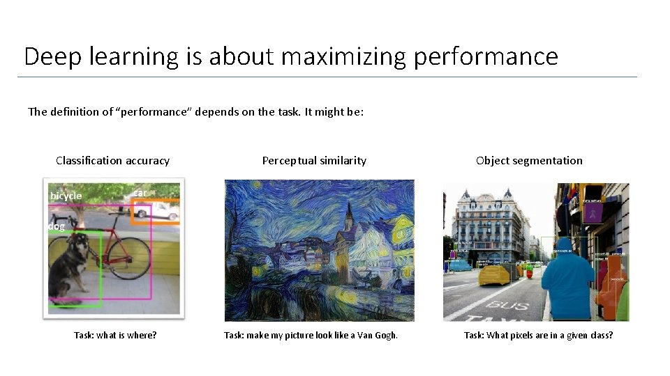
Deep learning is about maximizing performance The definition of “performance” depends on the task. It might be: Classification accuracy Perceptual similarity Task: what is where? Task: make my picture look like a Van Gogh. Object segmentation Task: What pixels are in a given class?

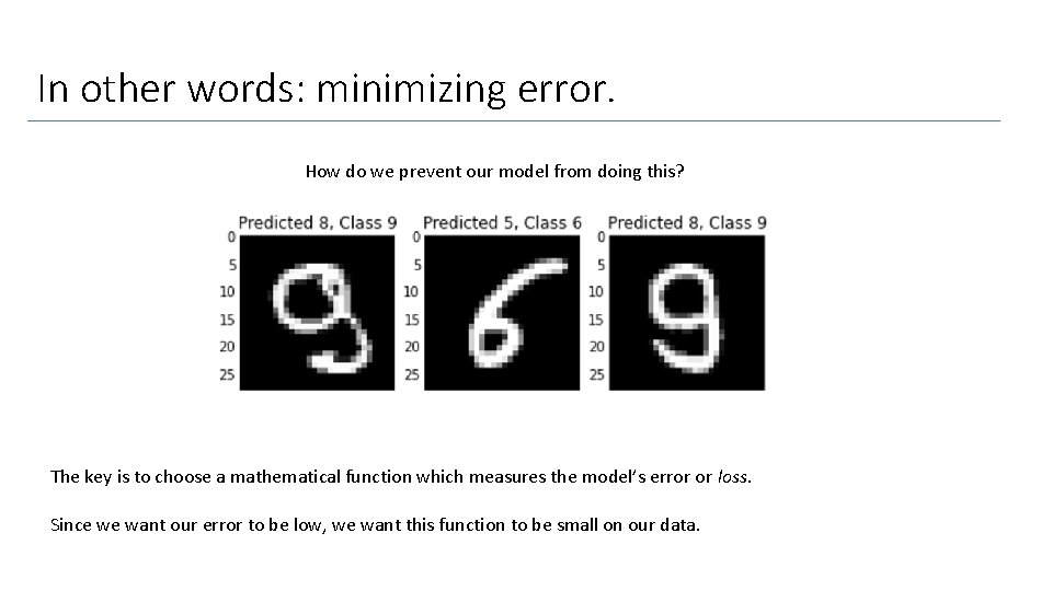
In other words: minimizing error. How do we prevent our model from doing this? The key is to choose a mathematical function which measures the model’s error or loss. Since we want our error to be low, we want this function to be small on our data.

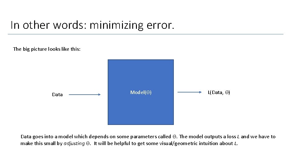
In other words: minimizing error. The big picture looks like this: Data Model(ϴ) L(Data, ϴ) Data goes into a model which depends on some parameters called ϴ. The model outputs a loss L and we have to make this small by adjusting ϴ. It will be helpful to get some visual/geometric intuition about L.

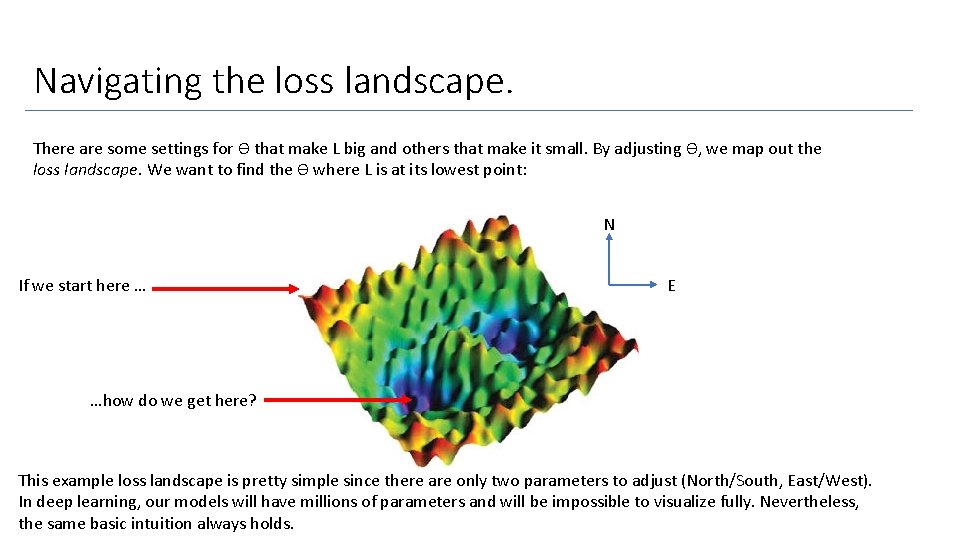
Navigating the loss landscape. There are some settings for ϴ that make L big and others that make it small. By adjusting ϴ, we map out the loss landscape. We want to find the ϴ where L is at its lowest point: N If we start here … E …how do we get here? This example loss landscape is pretty simple since there are only two parameters to adjust (North/South, East/West). In deep learning, our models will have millions of parameters and will be impossible to visualize fully. Nevertheless, the same basic intuition always holds.

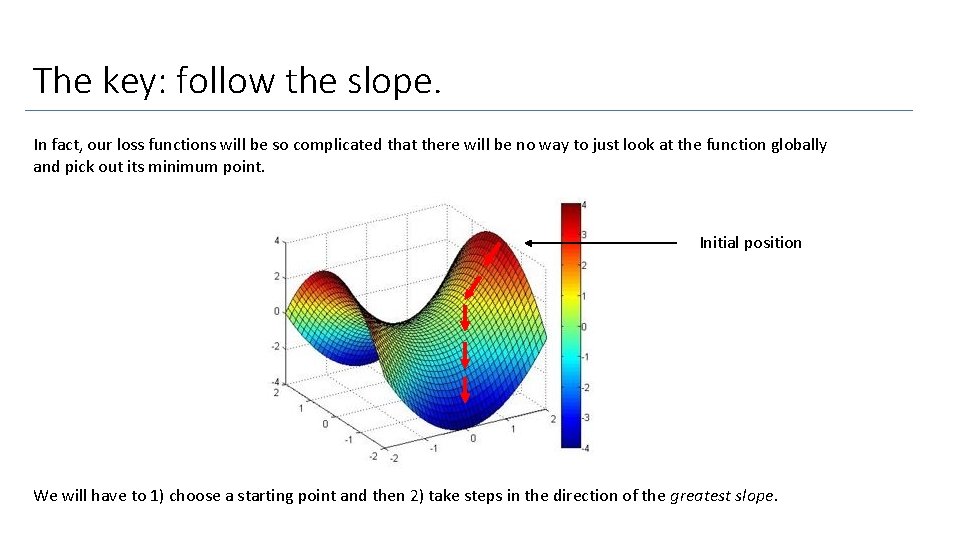
The key: follow the slope. In fact, our loss functions will be so complicated that there will be no way to just look at the function globally and pick out its minimum point. Initial position We will have to 1) choose a starting point and then 2) take steps in the direction of the greatest slope.

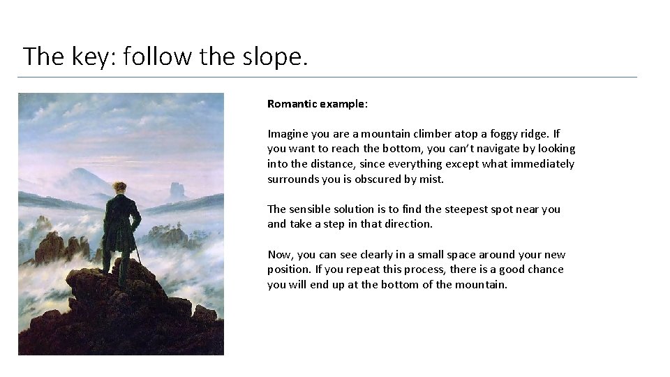
The key: follow the slope. Romantic example: Imagine you are a mountain climber atop a foggy ridge. If you want to reach the bottom, you can’t navigate by looking into the distance, since everything except what immediately surrounds you is obscured by mist. The sensible solution is to find the steepest spot near you and take a step in that direction. Now, you can see clearly in a small space around your new position. If you repeat this process, there is a good chance you will end up at the bottom of the mountain.

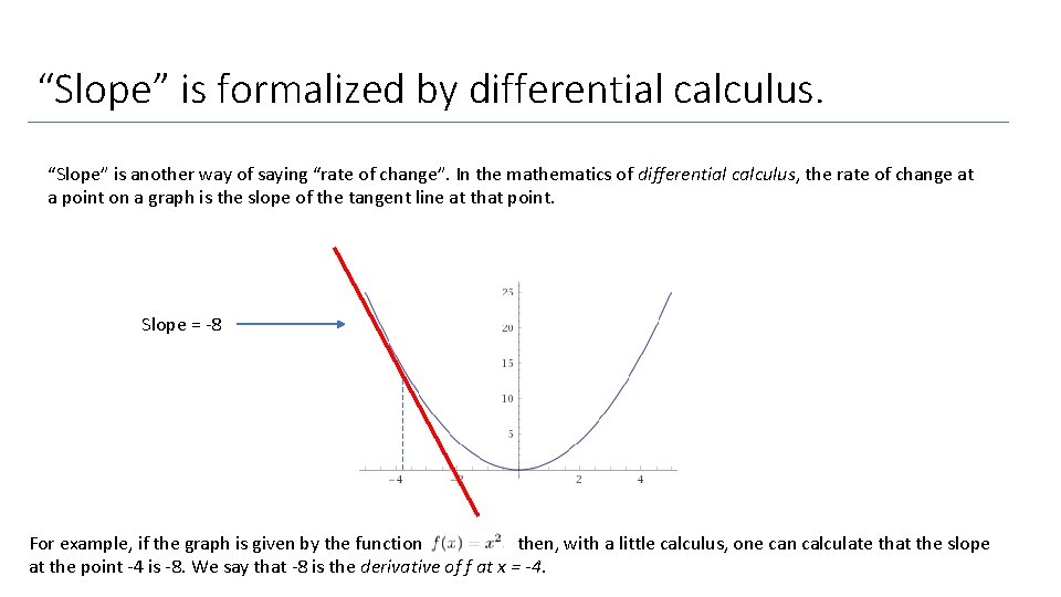
“Slope” is formalized by differential calculus. “Slope” is another way of saying “rate of change”. In the mathematics of differential calculus, the rate of change at a point on a graph is the slope of the tangent line at that point. Slope = -8 For example, if the graph is given by the function then, with a little calculus, one can calculate that the slope at the point -4 is -8. We say that -8 is the derivative of f at x = -4.

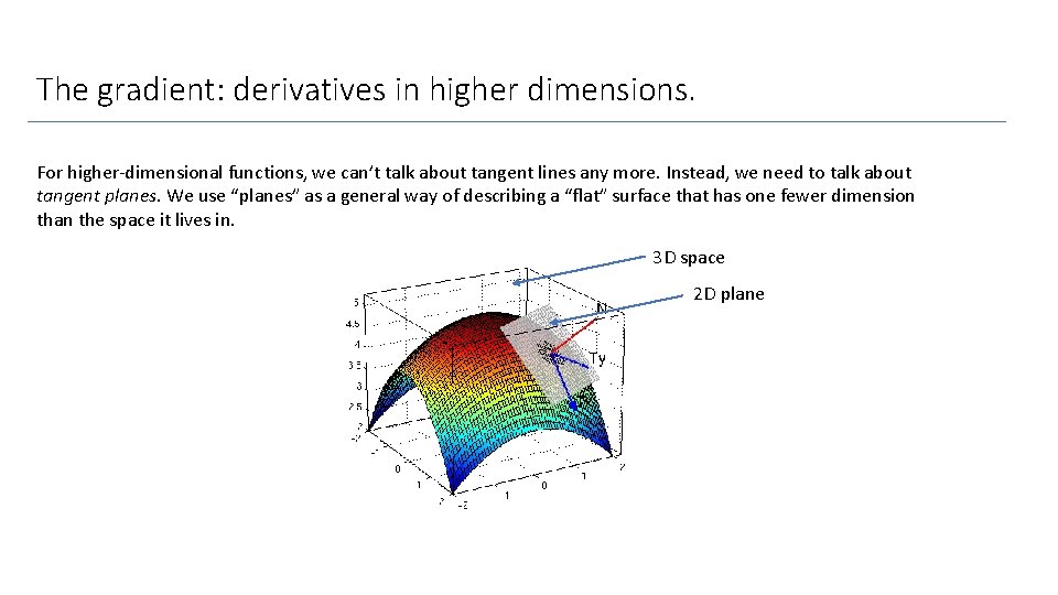
The gradient: derivatives in higher dimensions. For higher-dimensional functions, we can’t talk about tangent lines any more. Instead, we need to talk about tangent planes. We use “planes” as a general way of describing a “flat” surface that has one fewer dimension than the space it lives in. 3 D space 2 D plane

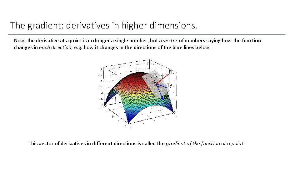
The gradient: derivatives in higher dimensions. Now, the derivative at a point is no longer a single number, but a vector of numbers saying how the function changes in each direction; e. g. how it changes in the directions of the blue lines below. This vector of derivatives in different directions is called the gradient of the function at a point.

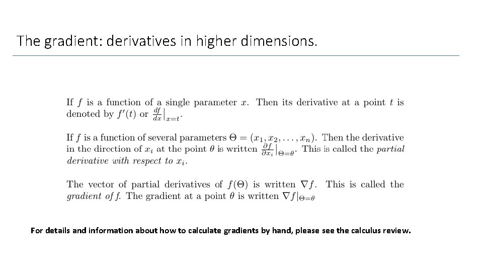
The gradient: derivatives in higher dimensions. For details and information about how to calculate gradients by hand, please see the calculus review.

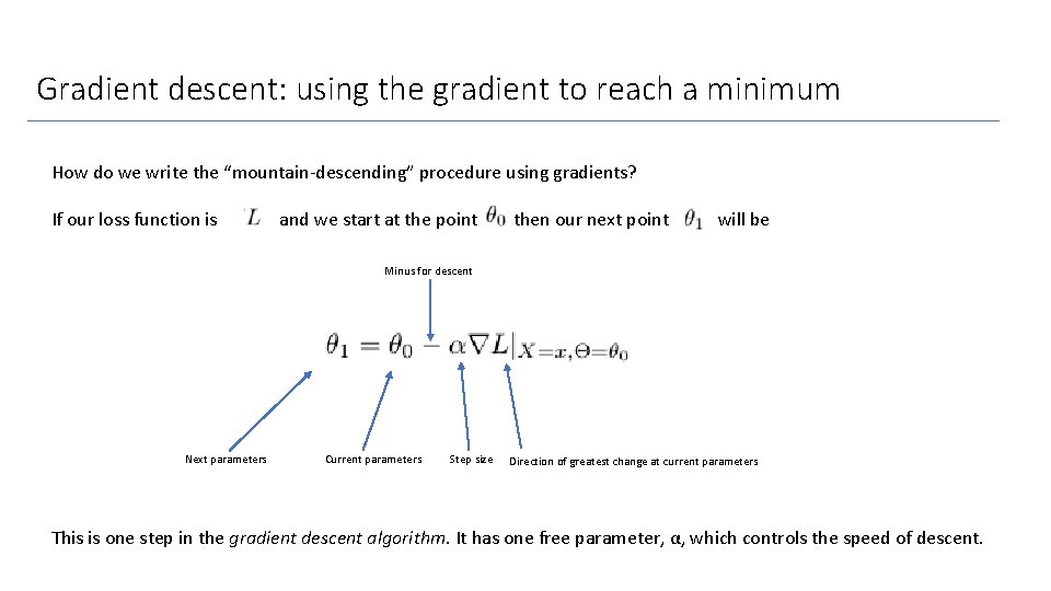
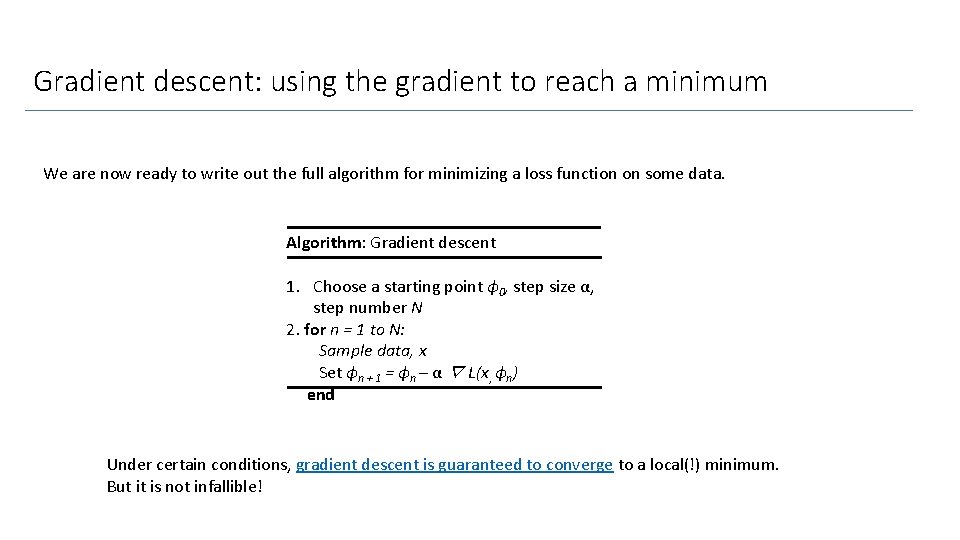
Gradient descent: using the gradient to reach a minimum How do we write the “mountain-descending” procedure using gradients? If our loss function is and we start at the point then our next point will be Minus for descent Next parameters Current parameters Step size Direction of greatest change at current parameters This is one step in the gradient descent algorithm. It has one free parameter, α, which controls the speed of descent.

Gradient descent: using the gradient to reach a minimum We are now ready to write out the full algorithm for minimizing a loss function on some data. Algorithm: Gradient descent 1. Choose a starting point ϕ 0, step size α, step number N 2. for n = 1 to N: Sample data, x Set ϕn + 1 = ϕn – α ∇ L(x, ϕn) end Under certain conditions, gradient descent is guaranteed to converge to a local(!) minimum. But it is not infallible!