GOVERNMENT POLICIES Economics 101 WHY GOVERNMENT POLICIES In

GOVERNMENT POLICIES Economics 101

WHY GOVERNMENT POLICIES? In a free, unregulated market system, market forces establish equilibrium prices and exchange quantities. While equilibrium conditions may be efficient, it may be true that not everyone is satisfied. One of the roles of economists is to use their theories to assist in the development of policies.

CONTROLS ON PRICES Are usually enacted when policymakers believe the market price is unfair to buyers or sellers. Result in government-created price ceilings and floors.

PRICE CEILING AND PRICE FLOOR Price Ceiling A legal maximum on the price at which a good can be sold. Price Floor A legal minimum on the price at which a good can be sold.

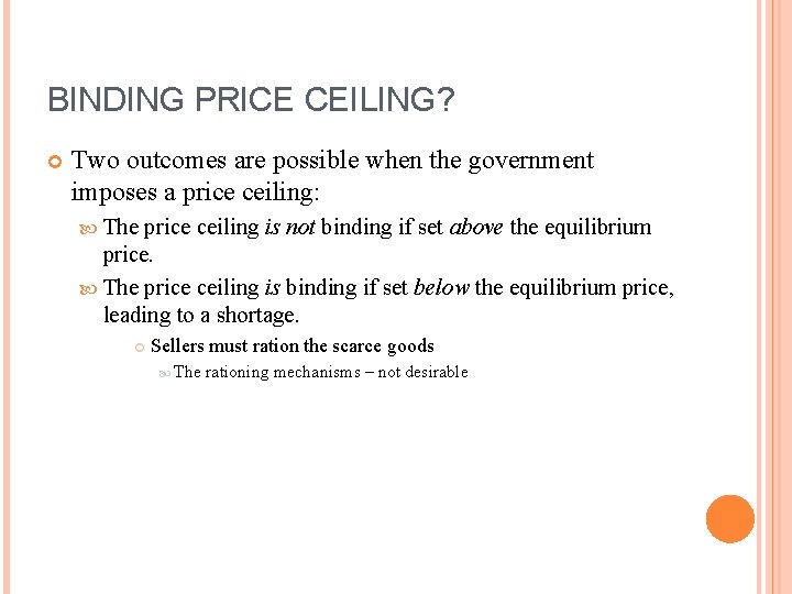
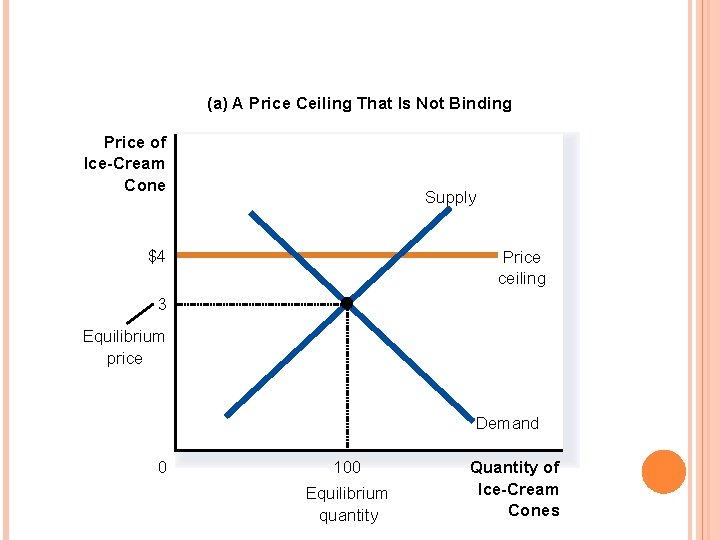
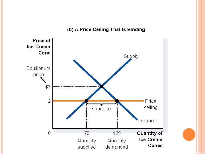
BINDING PRICE CEILING? Two outcomes are possible when the government imposes a price ceiling: The price ceiling is not binding if set above the equilibrium price. The price ceiling is binding if set below the equilibrium price, leading to a shortage. Sellers must ration the scarce goods The rationing mechanisms – not desirable

(a) A Price Ceiling That Is Not Binding Price of Ice-Cream Cone Supply $4 Price ceiling 3 Equilibrium price Demand 0 100 Equilibrium quantity Quantity of Ice-Cream Cones

(b) A Price Ceiling That Is Binding Price of Ice-Cream Cone Supply Equilibrium price $3 2 Price ceiling Shortage Demand 0 75 125 Quantity supplied Quantity demanded Quantity of Ice-Cream Cones Copyright© 2003 Southwestern/Thomson Learning

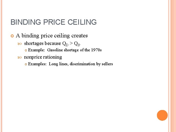
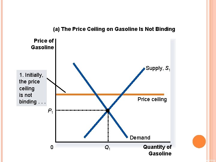
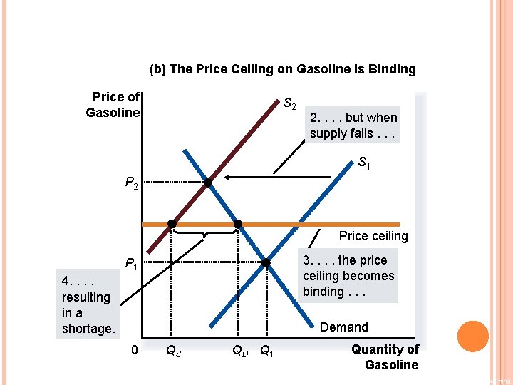
BINDING PRICE CEILING A binding price ceiling creates shortages because QD > QS. Example: Gasoline shortage of the 1970 s nonprice rationing Examples: Long lines, discrimination by sellers

CASE: LINES AT THE GAS PUMP In 1973, OPEC raised the price of crude oil in world markets. Crude oil is the major input in gasoline, so the higher oil prices reduced the supply of gasoline. What was responsible for the long gas lines?

(a) The Price Ceiling on Gasoline Is Not Binding Price of Gasoline Supply, S 1 1. Initially, the price ceiling is not binding. . . Price ceiling P 1 Demand 0 Q 1 Quantity of Gasoline Copyright© 2003 Southwestern/Thomson Learning

(b) The Price Ceiling on Gasoline Is Binding Price of Gasoline S 2 2. . but when supply falls. . . S 1 P 2 Price ceiling 3. . the price ceiling becomes binding. . . P 1 4. . resulting in a shortage. Demand 0 QS QD Q 1 Quantity of Gasoline Copyright© 2003 Southwestern/Thomson Learning

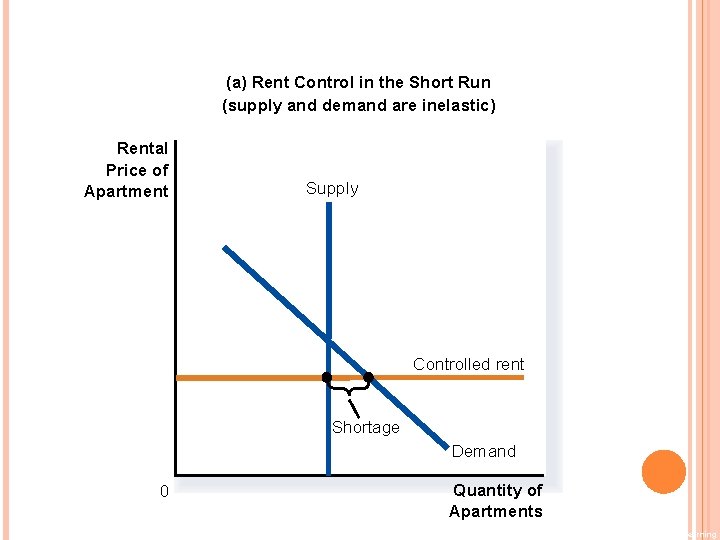
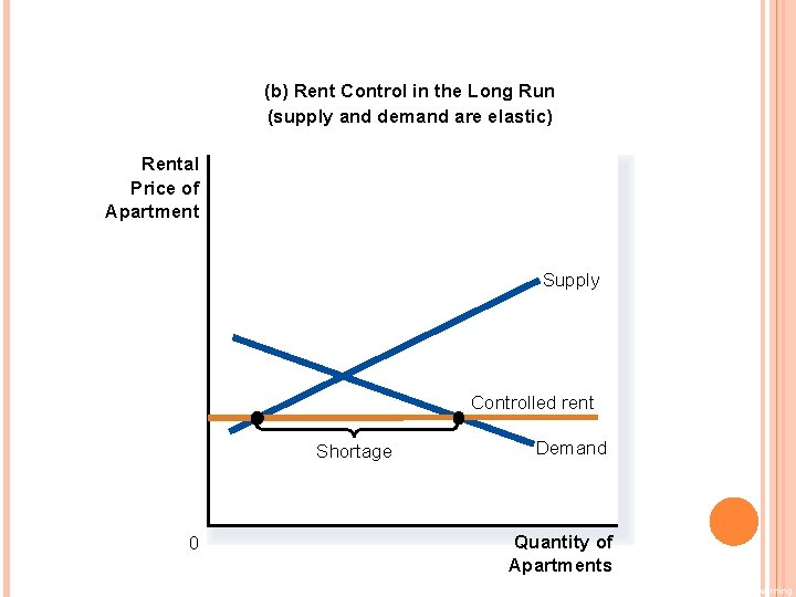
CASE: RENT CONTROL Rent controls are ceilings placed on the rents that landlords may charge their tenants. The goal of rent control policy is to help the poor by making housing more affordable. One economist called rent control “the best way to destroy a city, other than bombing. ”

(a) Rent Control in the Short Run (supply and demand are inelastic) Rental Price of Apartment Supply Controlled rent Shortage Demand 0 Quantity of Apartments Copyright© 2003 Southwestern/Thomson Learning

(b) Rent Control in the Long Run (supply and demand are elastic) Rental Price of Apartment Supply Controlled rent Shortage 0 Demand Quantity of Apartments Copyright© 2003 Southwestern/Thomson Learning

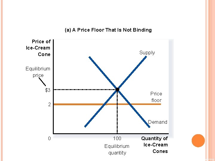
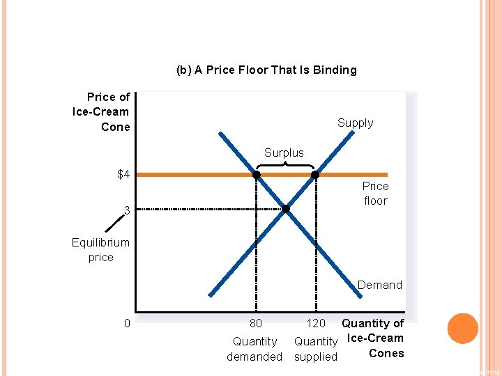
BINDING PRICE FLOOR? When the government imposes a price floor, two outcomes are possible. The price floor is not binding if set below the equilibrium price. The price floor is binding if set above the equilibrium price, leading to a surplus.

FIGURE 4 A MARKET WITH A PRICE FLOOR (a) A Price Floor That Is Not Binding Price of Ice-Cream Cone Supply Equilibrium price $3 Price floor 2 Demand 0 100 Equilibrium quantity Quantity of Ice-Cream Cones Copyright© 2003 Southwestern/Thomson Learning

FIGURE 4 A MARKET WITH A PRICE FLOOR (b) A Price Floor That Is Binding Price of Ice-Cream Cone Supply Surplus $4 Price floor 3 Equilibrium price Demand 0 Quantity of Quantity Ice-Cream Cones demanded supplied 80 120 Copyright© 2003 Southwestern/Thomson Learning

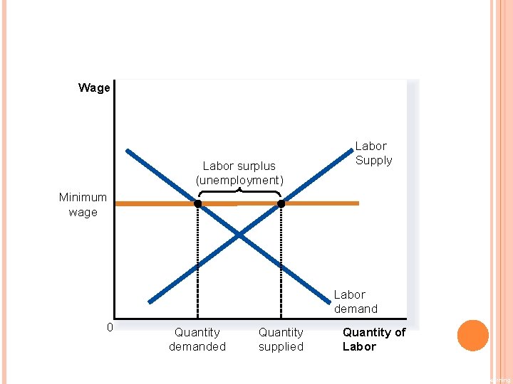
BINDING PRICE FLOOR A binding price floor causes. . . a surplus because QS > QD. nonprice rationing is an alternative mechanism for rationing the good, using discrimination criteria. Examples: The minimum wage, agricultural price supports

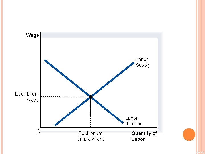
CASE: MINIMUM WAGE An important example of a price floor is the minimum wage. Minimum wage laws dictate the lowest price possible for labor that any employer may pay.

FIGURE 5 HOW THE MINIMUM WAGE AFFECTS THE LABOR MARKET Wage Labor Supply Equilibrium wage Labor demand 0 Equilibrium employment Quantity of Labor Copyright© 2003 Southwestern/Thomson Learning

FIGURE 5 HOW THE MINIMUM WAGE AFFECTS THE LABOR MARKET Wage Labor surplus (unemployment) Labor Supply Minimum wage Labor demand 0 Quantity demanded Quantity supplied Quantity of Labor Copyright© 2003 Southwestern/Thomson Learning

TAXES Governments levy taxes to raise revenue for public projects. Taxes discourage market activity. When a good is taxed (commodity tax), the quantity sold is smaller. Buyers and sellers share the tax burden.

TAX INCIDENCE Tax incidence is the manner in which the burden of a tax is shared among participants in a market. Tax incidence is the study of who bears the burden of a tax. _ Statutory incidence (legal incidence) _ Economic incidence

COMMODITY TAX Sale Tax Excise Tax

SALE TAX Sale Tax: a tax on buyer (statutory incidence) Example: USA Case: $0. 50 tax per ice-cream cone bought.

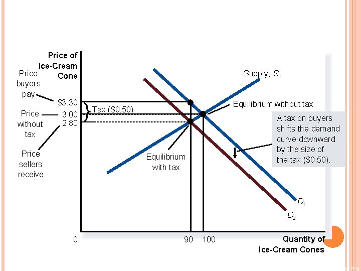
FIGURE 6 A TAX ON BUYERS Price of Ice-Cream Price Cone buyers pay $3. 30 Price 3. 00 2. 80 without tax Price sellers receive Supply, S 1 Equilibrium without tax Tax ($0. 50) A tax on buyers shifts the demand curve downward by the size of the tax ($0. 50). Equilibrium with tax D 1 D 2 0 90 100 Quantity of Ice-Cream Cones Copyright© 2003 Southwestern/Thomson Learning

WHO ACTUALLY BEARS THE TAX BURDEN? Buyers and sellers share the tax burden. (economic incidence) In this example, buyers share $0. 30 and sellers share $0. 20.

EXCISE TAX Excise Tax: A Tax on Seller (Statutory incidence) Example: Taiwan Case: $0. 50 tax per ice-cream cone sold

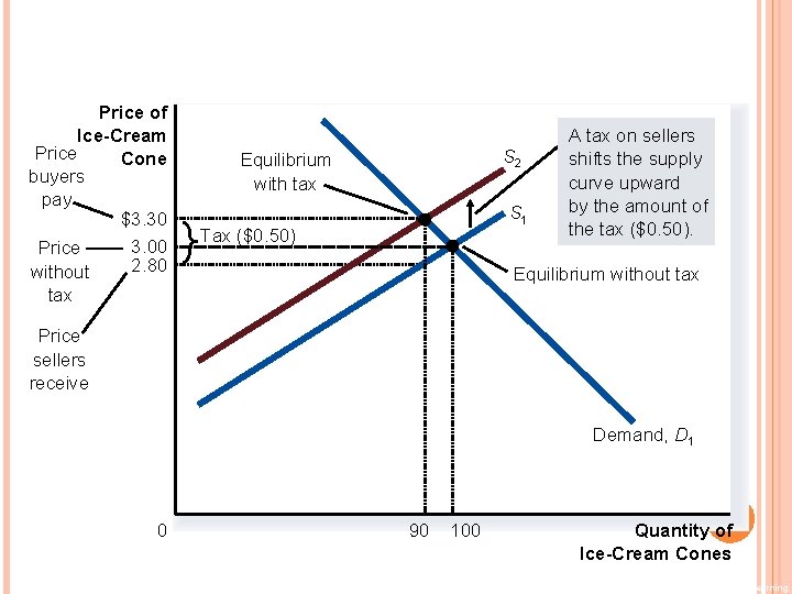
FIGURE 7 A TAX ON SELLERS Price of Ice-Cream Price Cone buyers pay $3. 30 3. 00 Price 2. 80 without tax S 2 Equilibrium with tax S 1 Tax ($0. 50) A tax on sellers shifts the supply curve upward by the amount of the tax ($0. 50). Equilibrium without tax Price sellers receive Demand, D 1 0 90 100 Quantity of Ice-Cream Cones Copyright© 2003 Southwestern/Thomson Learning

WHO ACTUALLY BEARS THE TAX BURDEN? Buyers and sellers share the tax burden. (economic incidence) In this example, buyers share $0. 30 and sellers share $0. 20.

ELASTICITY AND TAX INCIDENCE In what proportions is the burden of the tax divided? How do the effects of taxes on sellers compare to those levied on buyers? The answers to these questions depend on the elasticity of demand the elasticity of supply.

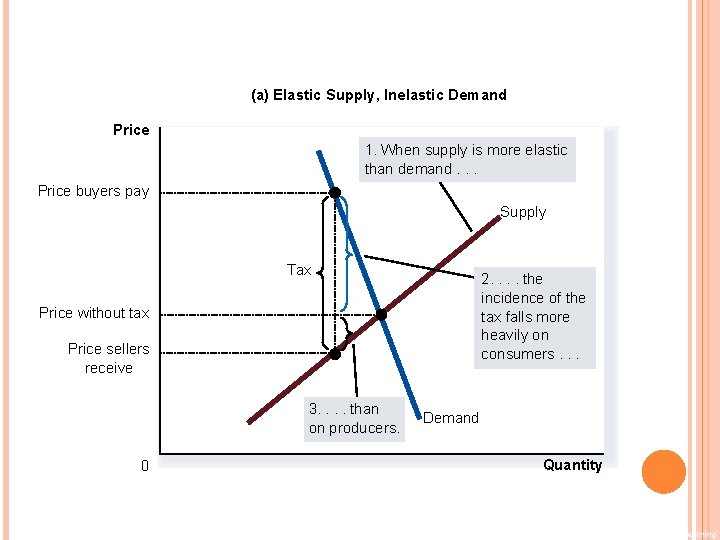
FIGURE 9 HOW THE BURDEN OF A TAX IS DIVIDED (a) Elastic Supply, Inelastic Demand Price 1. When supply is more elastic than demand. . . Price buyers pay Supply Tax 2. . the incidence of the tax falls more heavily on consumers. . . Price without tax Price sellers receive 3. . than on producers. 0 Demand Quantity Copyright© 2003 Southwestern/Thomson Learning

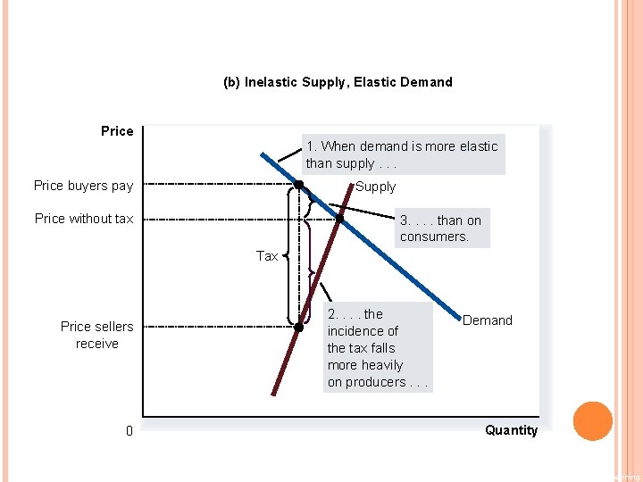
FIGURE 9 HOW THE BURDEN OF A TAX IS DIVIDED (b) Inelastic Supply, Elastic Demand Price 1. When demand is more elastic than supply. . . Price buyers pay Supply Price without tax 3. . than on consumers. Tax Price sellers receive 0 2. . the incidence of the tax falls more heavily on producers. . . Demand Quantity Copyright© 2003 Southwestern/Thomson Learning

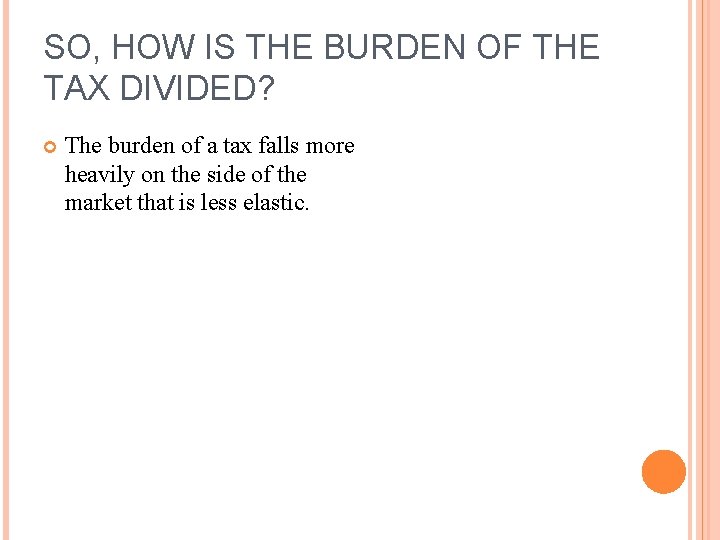
SO, HOW IS THE BURDEN OF THE TAX DIVIDED? The burden of a tax falls more heavily on the side of the market that is less elastic.

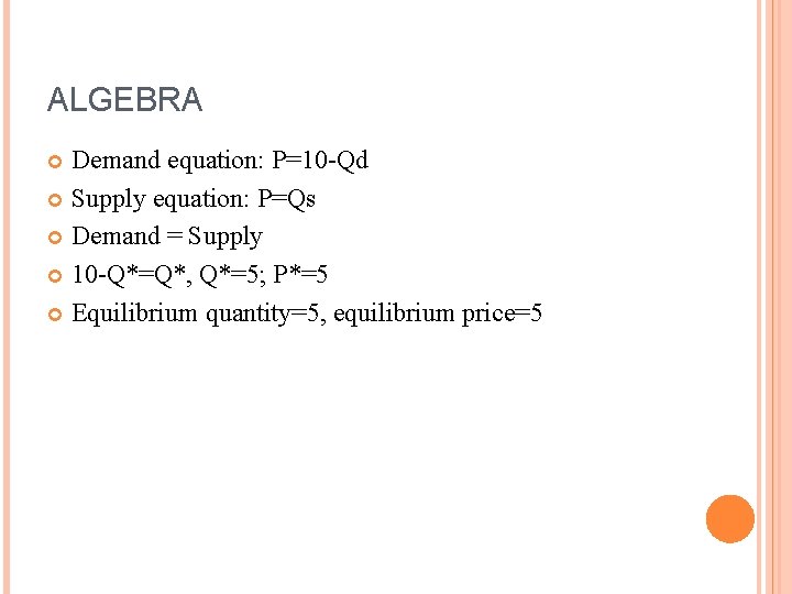
ALGEBRA Demand equation: P=10 -Qd Supply equation: P=Qs Demand = Supply 10 -Q*=Q*, Q*=5; P*=5 Equilibrium quantity=5, equilibrium price=5

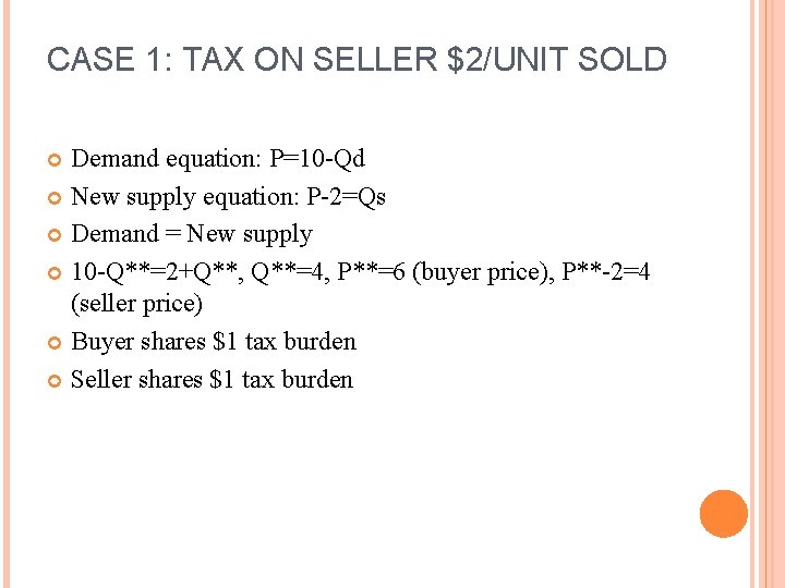
CASE 1: TAX ON SELLER $2/UNIT SOLD Demand equation: P=10 -Qd New supply equation: P-2=Qs Demand = New supply 10 -Q**=2+Q**, Q**=4, P**=6 (buyer price), P**-2=4 (seller price) Buyer shares $1 tax burden Seller shares $1 tax burden

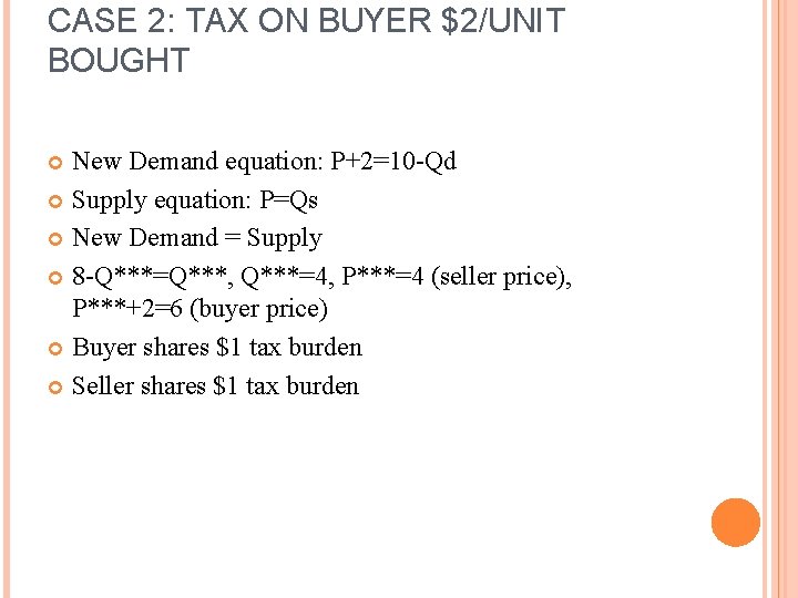
CASE 2: TAX ON BUYER $2/UNIT BOUGHT New Demand equation: P+2=10 -Qd Supply equation: P=Qs New Demand = Supply 8 -Q***=Q***, Q***=4, P***=4 (seller price), P***+2=6 (buyer price) Buyer shares $1 tax burden Seller shares $1 tax burden

QUIZ Demand is perfectly inelastic and supply is elastic 1. Tax on buyers (sales tax) 2. Tax on sellers (excise tax)

QUIZ Supply is perfectly inelastic and demand is elastic 1. Tax on buyers (sales tax) 2. Tax on sellers (excise tax)