Goodfellow Chapter 9 Convolutional Networks Dr Charles Tappert

Goodfellow: Chapter 9 Convolutional Networks Dr. Charles Tappert The information here, although greatly condensed, comes almost entirely from the chapter content.

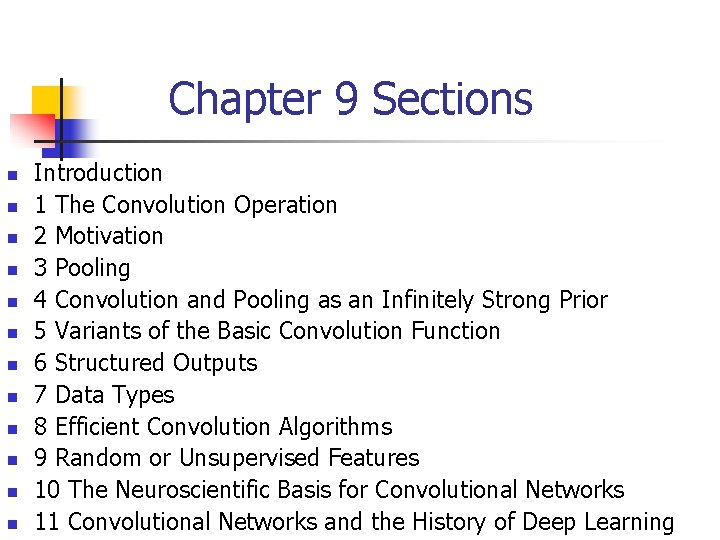
Chapter 9 Sections n n n Introduction 1 The Convolution Operation 2 Motivation 3 Pooling 4 Convolution and Pooling as an Infinitely Strong Prior 5 Variants of the Basic Convolution Function 6 Structured Outputs 7 Data Types 8 Efficient Convolution Algorithms 9 Random or Unsupervised Features 10 The Neuroscientific Basis for Convolutional Networks 11 Convolutional Networks and the History of Deep Learning

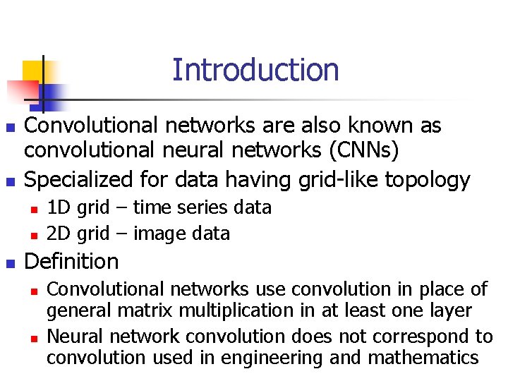
Introduction n n Convolutional networks are also known as convolutional neural networks (CNNs) Specialized for data having grid-like topology n n n 1 D grid – time series data 2 D grid – image data Definition n n Convolutional networks use convolution in place of general matrix multiplication in at least one layer Neural network convolution does not correspond to convolution used in engineering and mathematics

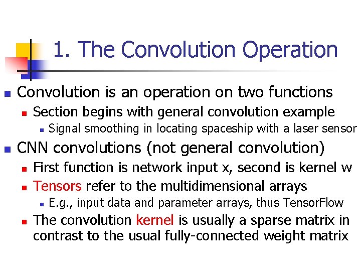
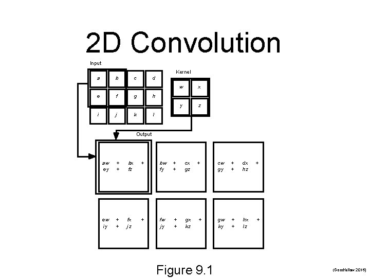
1. The Convolution Operation n Convolution is an operation on two functions n Section begins with general convolution example n n Signal smoothing in locating spaceship with a laser sensor CNN convolutions (not general convolution) n n First function is network input x, second is kernel w Tensors refer to the multidimensional arrays n n E. g. , input data and parameter arrays, thus Tensor. Flow The convolution kernel is usually a sparse matrix in contrast to the usual fully-connected weight matrix

2 D Convolution Input Kernel a b e c f i d g j w x y z h k l Output aw ey + + bx fz + bw fy + + cx gz + cw gy + + dx hz + ew iy + + fx jz + fw jy + + gx kz + gw ky + + hx lz + Figure 9. 1 (Goodfellow 2016)

2. Motivation n Convolution leverages three important ideas that help improve machine learning systems 1. 2. 3. Sparse interactions Parameter sharing Equivariant representations

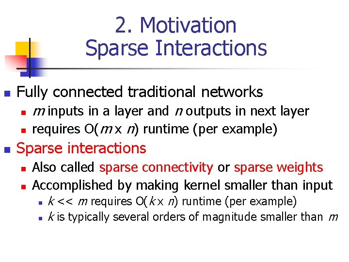
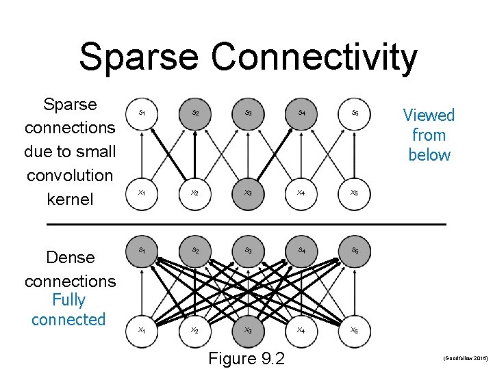
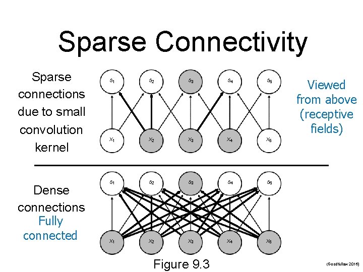
2. Motivation Sparse Interactions n Fully connected traditional networks n n n m inputs in a layer and n outputs in next layer requires O(m x n) runtime (per example) Sparse interactions n n Also called sparse connectivity or sparse weights Accomplished by making kernel smaller than input n n k << m requires O(k x n) runtime (per example) k is typically several orders of magnitude smaller than m

Sparse Connectivity Sparse connections due to small convolution kernel Dense connections Fully connected s 1 s 2 s 3 s 4 s 5 x 1 x 2 x 3 x 4 x 5 Figure 9. 2 Viewed from below (Goodfellow 2016)

Sparse Connectivity Sparse connections due to small convolution kernel Dense connections Fully connected s 1 s 2 s 3 s 4 s 5 x 1 x 2 x 3 x 4 x 5 Figure 9. 3 Viewed from above (receptive fields) (Goodfellow 2016)

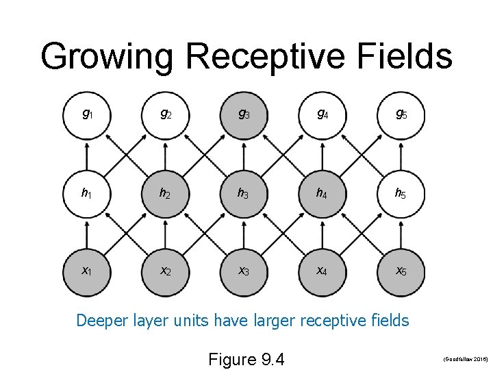
Growing Receptive Fields g 1 g 2 g 3 g 4 g 5 h 1 h 2 h 3 h 4 h 5 x 1 x 2 x 3 x 4 x 5 Deeper layer units have larger receptive fields Figure 9. 4 (Goodfellow 2016)

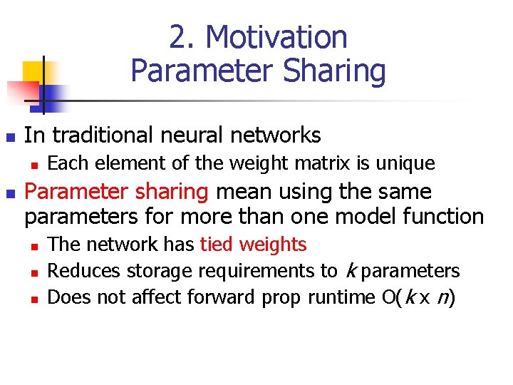
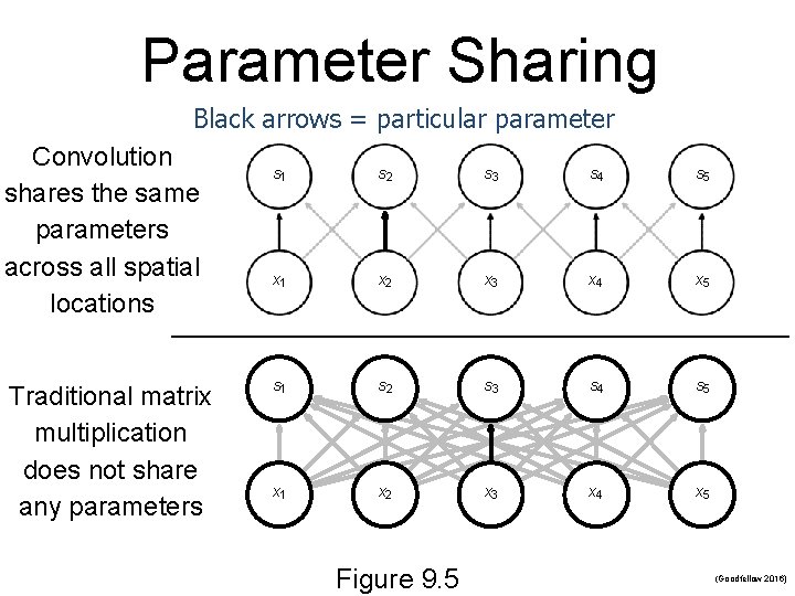
2. Motivation Parameter Sharing n In traditional neural networks n n Each element of the weight matrix is unique Parameter sharing mean using the same parameters for more than one model function n The network has tied weights Reduces storage requirements to k parameters Does not affect forward prop runtime O(k x n)

Parameter Sharing Black arrows = particular parameter Convolution shares the same parameters across all spatial locations Traditional matrix multiplication does not share any parameters s 1 s 2 s 3 s 4 s 5 x 1 x 2 x 3 x 4 x 5 Figure 9. 5 (Goodfellow 2016)

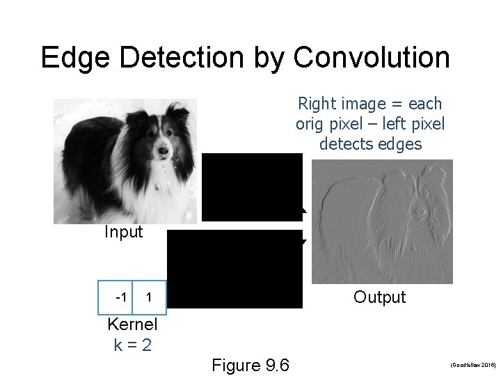
Edge Detection by Convolution Right image = each orig pixel – left pixel detects edges Input -1 Output 1 Kernel k=2 Figure 9. 6 (Goodfellow 2016)

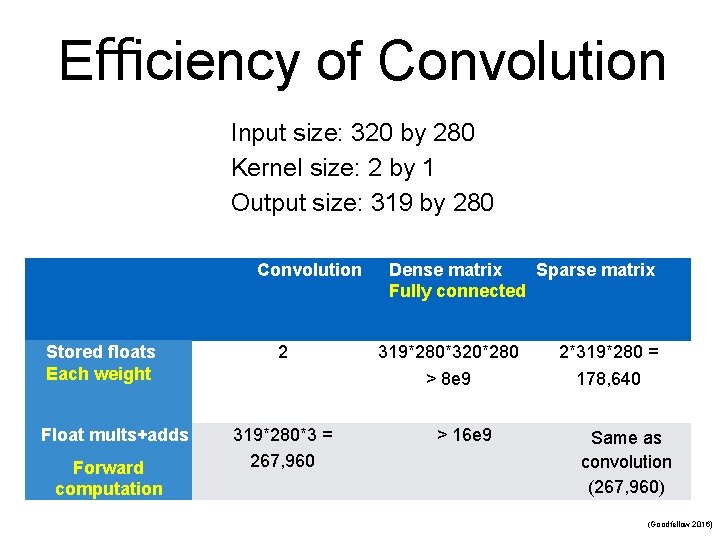
Efficiency of Convolution Input size: 320 by 280 Kernel size: 2 by 1 Output size: 319 by 280 Convolution Stored floats Each weight Float mults+adds Forward computation 2 319*280*3 = 267, 960 Dense matrix Sparse matrix Fully connected 319*280*320*280 > 8 e 9 > 16 e 9 2*319*280 = 178, 640 Same as convolution (267, 960) (Goodfellow 2016)

2. Motivation Equivariant Representations n n For an invariant function, if the input changes, the output change in the same way For convolution, a particular form of parameter sharing causes equivariance to translation n n For example, as the dog moves in the input image, the detected edges move in the same way In image processing, detecting edges is useful in the first layer, and edges appear more or less everywhere in the image

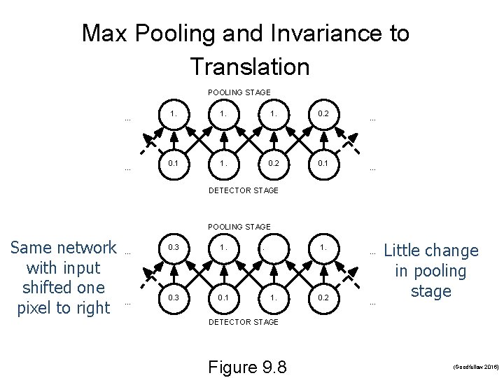
3. Pooling n The pooling function replaces the output of the net at a certain location with a summary statistic of the nearby outputs n n n Max pooling reports the maximum output within a rectangular neighborhood Average pooling reports the average output Pooling helps make the representation approximately invariant to small input translations

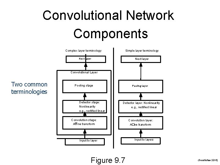
Convolutional Network Components Complex layer terminology Simple layer terminology Next layer Convolutional Layer Two common terminologies Pooling stage Detector stage: Nonlinearity e. g. , rectified linear Pooling layer Detector layer: Nonlinearity e. g. , rectified linear Convolution stage: Affine transform Convolution layer: A�ne transform Input to layers Figure 9. 7 (Goodfellow 2016)

Max Pooling and Invariance to Translation POOLING STAGE. . . 1. 1. 0. 2 0. 1 . . . DETECTOR STAGE POOLING STAGE Same network with input shifted one pixel to right . . . 0. 3 1. 0. 3 0. 1 1. 1. 0. 2 . . . Little change in pooling stage DETECTOR STAGE Figure 9. 8 (Goodfellow 2016)

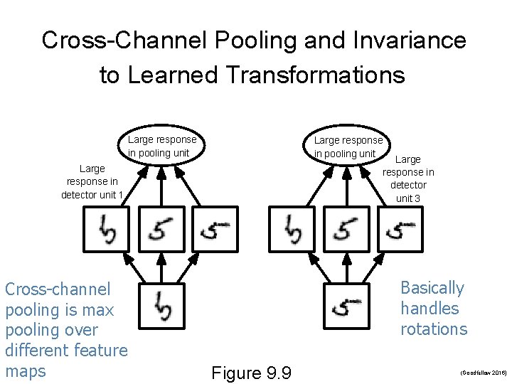
Cross-Channel Pooling and Invariance to Learned Transformations Large response in pooling unit Large response in detector unit 3 Large response in detector unit 1 Cross-channel pooling is max pooling over different feature maps Basically handles rotations Figure 9. 9 (Goodfellow 2016)

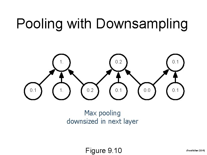
Pooling with Downsampling 1. 0. 1 1. 0. 2 0. 1 0. 0 0. 1 Max pooling downsized in next layer Figure 9. 10 (Goodfellow 2016)

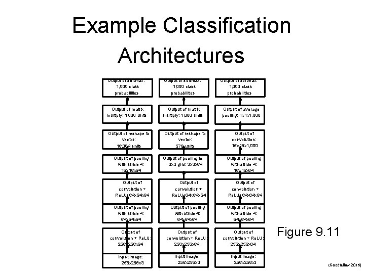
Example Classification Architectures Output of softmax: 1, 000 class probabilities Output of matrix multiply: 1, 000 units Output of reshape to vector: 16, 384 units Output of pooling with stride 4: 16 x 64 Output of reshape to vector: 576 units Output of pooling to 3 x 3 grid: 3 x 3 x 64 Output of softmax: 1, 000 class probabilities Output of average pooling: 1 x 1 x 1, 000 Output of convolution: 16 x 1, 000 Output of pooling with stride 4: 16 x 64 Output of convolution + Re. LU: 64 x 64 x 64 Output of pooling with stride 4: 64 x 64 Output of convolution + Re. LU: 256 x 64 Output of convolution + Re. LU: 256 x 64 Input image: 256 x 3 Input image: 256 x 3 Figure 9. 11 (Goodfellow 2016)

4. Convolution and Pooling as an Infinitely Strong Prior n Prior probabilities (beliefs before we see actual data) can be strong or weak n n A weak prior (e. g. , Gaussian distribution with high variance) allows the data to move the parameters A strong prior (e. g. , Gaussian distribution with low variance) strongly determines the parameters An infinitely strong prior controls the parameters A convolutional net ~ an infinitely strong prior n n Weights are zero except in small receptive fields Weights identical for neighboring hidden units

4. Convolution and Pooling as an Infinitely Strong Prior n Convolution and pooling can cause underfitting n n n The prior is useful only when the assumptions made by the prior are reasonably accurate If a task relies on preserving precise spatial information, then pooling can increase training error The prior imposed by convolution must be appropriate

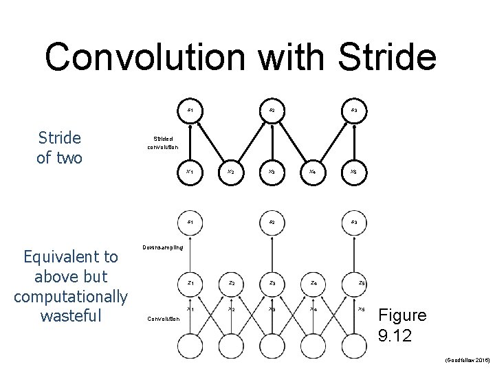
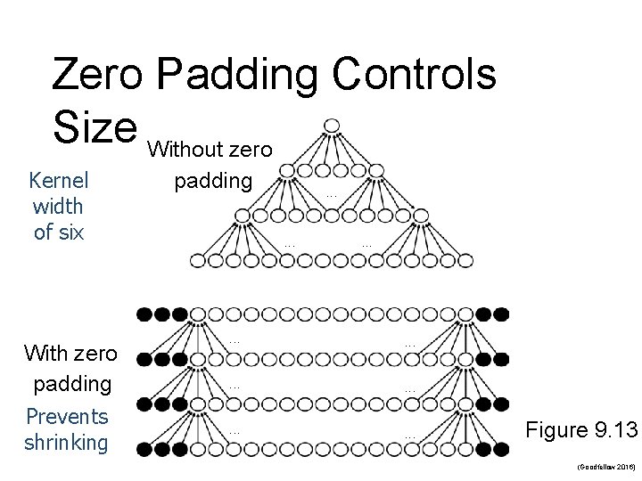
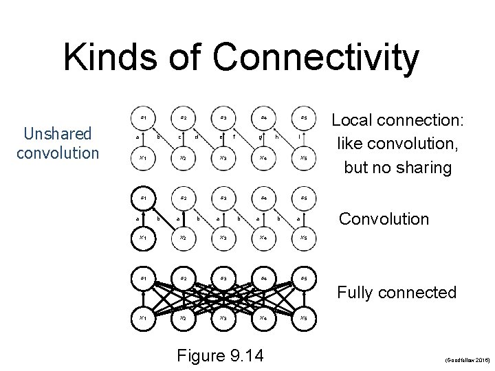
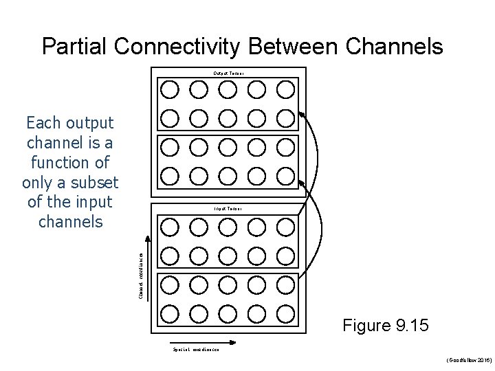
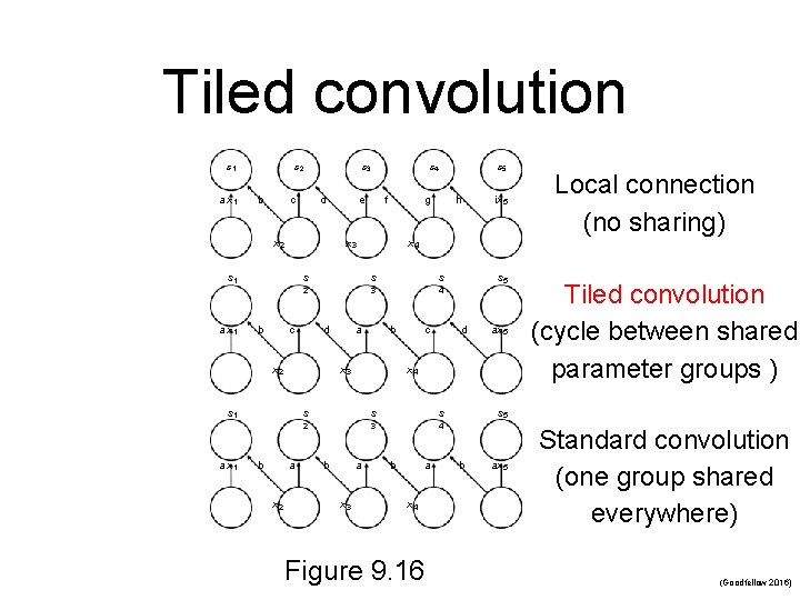
5. Variants of the Basic Convolution Function n Stride is the amount of downsampling n n n Zero padding avoids layer-to-layer shrinking Unshared convolution n Can have separate strides in different directions Like convolution but without sharing Partial connectivity between channels Tiled convolution n Cycle between shared parameter groups

Convolution with Stride s 1 Stride of two s 2 Strided convolution x 1 x 2 s 1 Equivalent to above but computationally wasteful s 3 x 4 s 2 x 5 s 3 Downsampling Convolution z 1 z 2 z 3 z 4 z 5 x 1 x 2 x 3 x 4 x 5 Figure 9. 12 (Goodfellow 2016)

Zero Padding Controls Size Without zero Kernel width of six With zero padding Prevents shrinking padding . . . . Figure 9. 13 (Goodfellow 2016)

Kinds of Connectivity s 1 Unshared convolution a s 2 b c s 3 d e s 4 f g s 5 h i x 1 x 2 x 3 x 4 x 5 s 1 s 2 s 3 s 4 s 5 a b a b Local connection: like convolution, but no sharing Convolution a x 1 x 2 x 3 x 4 x 5 s 1 s 2 s 3 s 4 s 5 Fully connected x 1 x 2 x 3 x 4 Figure 9. 14 x 5 (Goodfellow 2016)

Partial Connectivity Between Channels Output Tensor Each output channel is a function of only a subset of the input channels Channel coordinates Input Tensor Figure 9. 15 Spatial coordinates (Goodfellow 2016)

Tiled convolution s 1 a x 1 s 2 b c s 3 d x 2 b s 3 4 a x 2 a b x 3 s 1 c ax 5 x 4 s s 2 3 4 a x 3 s 5 d s b ix 5 Local connection (no sharing) x 4 s d s 5 h 2 c b g s x 2 a x 1 f x 3 s 1 a x 1 e s 4 b a x 4 Figure 9. 16 Tiled convolution (cycle between shared parameter groups ) s 5 b ax 5 Standard convolution (one group shared everywhere) (Goodfellow 2016)

6. Structured Outputs n n Convolutional networks are usually used for classification They can also be used to output a highdimensional, structured object n The object is typically a tensor

7. Data Types n Single channel examples: n n 1 D audio waveform 2 D audio data after Fourier transform n n Frequency versus time Multi-channel examples: n 2 D color image data n n Three channels: red pixels, green pixels, blue pixels Each channel is 2 D for the image

8. Efficient Convolution Algorithms n n Devising faster ways of performing convolution or approximate convolution without harming the accuracy of the model is an active area of research However, most dissertation work concerns feasibility and not efficiency

9. Random or Unsupervised Features n n One way to reduce the cost of convolutional network training is to use features that are not trained in a supervised fashion Three methods (Rosenblatt used first two) 1. 2. 3. Simply initialize convolutional kernels randomly Design them by hand Learn the kernels using unsupervised methods

10. The Neuroscientific Basis for Convolutional Networks n n Convolutional networks may be the greatest success story of biologically inspired AI Some of the key design principles of neural networks were drawn from neuroscience n Hubel and Wiesel won the Nobel prize in 1981 for their work on the cat’s visual system 1960 s-1970 s

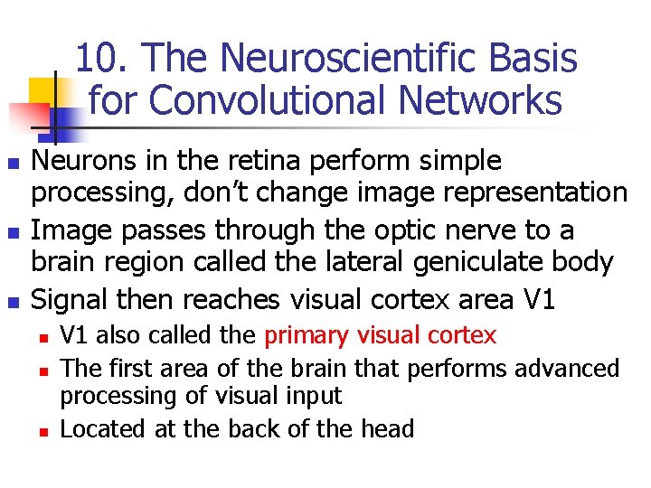
10. The Neuroscientific Basis for Convolutional Networks n n n Neurons in the retina perform simple processing, don’t change image representation Image passes through the optic nerve to a brain region called the lateral geniculate body Signal then reaches visual cortex area V 1 n n n V 1 also called the primary visual cortex The first area of the brain that performs advanced processing of visual input Located at the back of the head

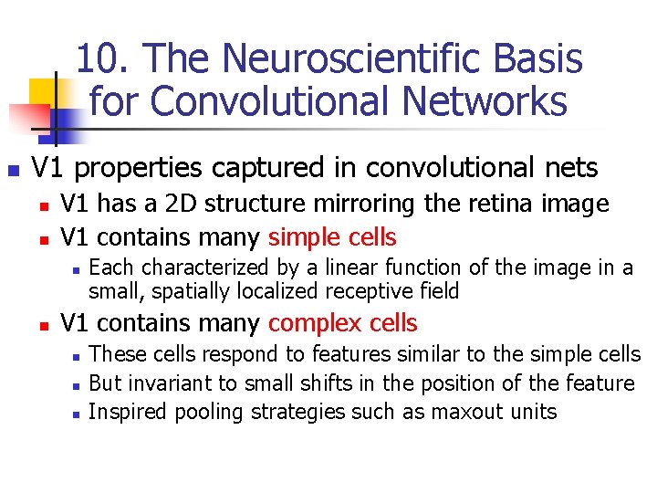
10. The Neuroscientific Basis for Convolutional Networks n V 1 properties captured in convolutional nets n n V 1 has a 2 D structure mirroring the retina image V 1 contains many simple cells n n Each characterized by a linear function of the image in a small, spatially localized receptive field V 1 contains many complex cells n n n These cells respond to features similar to the simple cells But invariant to small shifts in the position of the feature Inspired pooling strategies such as maxout units

10. The Neuroscientific Basis for Convolutional Networks n Although we know most about area V 1, we believe similar principles apply to other areas n n Basic strategy of detection followed by pooling Passing through deeper layers, we find cells responding to specific concepts n These cells are nicknamed “grandmother cells” n The idea being that a neuron activates upon seeing their grandmother anywhere in the image

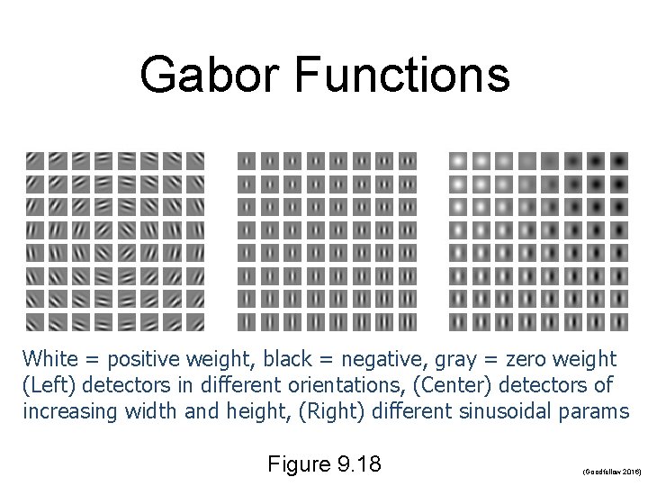
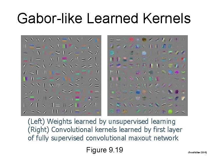
10. The Neuroscientific Basis for Convolutional Networks n Reverse correlation n n In biological networks we don’t have access to the weights themselves However, we can put an electrode in a neuron, display images in front of the animal’s retina, and record the activation of the neuron We can then fit a linear model to these responses to approximate the neuron’s weights Most V 1 cells have weights of Gabor functions

Gabor Functions White = positive weight, black = negative, gray = zero weight (Left) detectors in different orientations, (Center) detectors of increasing width and height, (Right) different sinusoidal params Figure 9. 18 (Goodfellow 2016)

Gabor-like Learned Kernels (Left) Weights learned by unsupervised learning (Right) Convolutional kernels learned by first layer of fully supervised convolutional maxout network Figure 9. 19 (Goodfellow 2016)

11. Convolutional Networks and the History of Deep Learning n Convolutional networks have played an important role in the history of deep learning n n n Application of neuroscience to machine learning First deep models to perform well First important commercial applications Used to win many contests Some of first deep networks trained with back-prop Performed well decades ago to pave the way toward acceptance of neural networks in general

11. Convolutional Networks and the History of Deep Learning n Convolutional networks allow specialized neural networks for grid-structured topology n n Most successful on 2 D image topology For 1 D sequential data we use recurrent networks