Goals Aims and Requirements Goals and aims To


")
 You have already defined the target")
")
 You next tell Excel which cells are")
")


 Constraints Non-Binding (or Inactive) Constraints Redundant Constraints")


 • What is the")
 • If the coefficient")
 • If the right-hand")

 • If the objective")

 S (supply)")


- Slides: 85
Goals, Aims, and Requirements Goals and aims To introduce Linear Programming To find a knowledge on graphical solution for LP problems To solve linear programming problems using excel.
The Lego Production Problem You have a set of logos 8 small bricks 6 large bricks These are your “raw materials”. You have to produce tables and chairs out of these logos. These are your “products”.
The Lego Production Problem Weekly supply of raw materials: 8 Small Bricks 6 Large Bricks Products: Table Profit = $20/Table Chair Profit = $15/Chair
Problem Formulation X 1 is the number of Chairs X 2 is the number of Tables Large brick constraint X 1+2 X 2 <= 6 Small brick constraint 2 X 1+2 X 2 <= 8 Objective function is to Maximize 15 X 1+20 X 2 X 1>=0 X 2>= 0
Graphical Solution to the Prototype Problem Tables 5 4 3 2 X 1 + 2 X 2 = 6 Large Bricks 1 0 1 2 3 4 5 6 Chairs
Graphical Solution to the Prototype Problem Tables 5 4 2 X 1 + 2 X 2 = 8 Small Bricks 3 2 1 0 1 2 3 4 5 6 Chairs
Graphical Solution to the Prototype Problem Tables 5 4 2 X 1 + 2 X 2 = 8 Small Bricks 3 2 X 1 + 2 X 2 = 6 Large Bricks 1 0 1 2 3 4 5 6 Chairs
Graphical Solution to the Prototype Problem Tables 5 4 3 X 1 + 2 X 2 = 6 Large Bricks 2 2 X 1 + 2 X 2 = 8 Small Bricks 1 0 1 2 3 4 5 6 Chairs
The Objective Function Z = 15 X 1 + 20 X 2 Lets draw it for 15 X 1 + 20 X 2 = 30 In this case if # of chair = 0, then # of table = 30/20 = 1. 5 if # of table = 0, then # of chair = 30/15 = 2
Graphical Solution to the Prototype Problem Tables 5 4 3 X 1 + 2 X 2 = 6 Large Bricks 2 2 X 1 + 2 X 2 = 8 Small Bricks 1 0 1 2 3 4 5 6 Chairs
A second example We can make Product 1 and or Product 2. There are 3 resources; Resource 1, Resource 2, Resource 3. Product 1 needs one unit of Resource 1, nothing of Resource 2, and three units of resource 3. Product 2 needs nothing from Resource 1, two units of Resource 2, and two units of resource 3. Available amount of resources 1, 2, 3 are 4, 12, 18, respectively. Net profit of product 1 and Product 2 are 3 and 5, respectively. • Formulate the Problem • Solve it graphically • Solve it using excel.
Problem 2 Product 1 needs 1 hour of Plant 1, and 3 hours of Plant 3. Product 2 needs 2 hours of plant 2 and 2 hours of plant 3 There are 4 hours available in plant 1, 12 hours in plant 2, and 18 hours in plant 3 Objective Function Z = 3 x 1 +5 x 2 Constraints Resource 1 x 1 4 Resource 2 2 x 2 12 Resource 3 3 x 1 + 2 x 2 18 Nonnegativity x 1 0, x 2 0
Problem 2 : Original version Max Z = 3 x 1 + 5 x 2 Subject to x 1 4 2 x 2 12 3 x 1 + 2 x 2 18 x 1 0, x 2 0 x 2 10 9 8 7 6 5 4 3 2 1 1 2 3 4 5 6 7 8 9 10 x 1
Problem 2 Max Z = 3 x 1 + 5 x 2 Subject to x 1 4 2 x 2 12 3 x 1 + 2 x 2 18 x 1 0, x 2 0 x 2 10 9 8 7 6 5 4 3 2 1 1 2 3 4 5 6 7 8 9 10 x 1
Implementing LP Models in Excel 1. Start by Organizing the data for the model on the spreadsheet. Type in the coefficients of the constraints and the objective function 2. For each constraint, create a formula in a separate cell that corresponds to the left-hand side (LHS) of the constraint. 3. Assign a set of cells to represent the decision variable in the model. 4. Create a formula in a cell that corresponds to the objective function.
Constraint LHS, Variables, Objective Function • Constraint cells - the cells in the spreadsheet representing the LHS formulas on the constraints • Changing cells - the cells in the spreadsheet representing the decision variables • Target cell - the cell in the spreadsheet that represents the objective function
Solving LP Models with Excel Enter the input data and construct relationships among data elements in a readable, easy to understand way. Make sure there is a cell in your spreadsheet for each of the following: ü every quantity that you might want to constraint (include both sides of the constraint) ü every decision variable ü the quantity you wish to maximize or minimize Usually we don’t have any particular initial values for the decision variables. The problem starts with assuming a value of 0 in each decision variable cell.
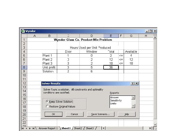
Wyndor Example Product 1 needs 1 hour of Plant 1, and 3 hours of Plant 3. Product 2 needs 2 hours of plant 2 and 2 hours of plant 3 There are 4 hours available in plant 1, 12 hours in plant 2, and 18 hours in plant 3 Z = 3 x 1 +5 x 2 x 1 4 2 x 2 12 3 x 1 + 2 x 2 18 x 1 0, x 2 0 Go to EXCEL, solve this problem in EXCEL first
Wyndor Example; Enter data
Noncomputational Entries
Sumproduct SUMPRODUCT function is used to multiply element by element of two tables and addup all values. In EXCELterminology, SUMPRODUCT sums the products of individual cells in two ranges. For example, SUMPRODUCT(C 6: D 6, C 4: D 4) sums the products C 6*C 4 plus D 6*D 4. The two specified ranges must be of the same size ( the same number of rows and columns). For linear programming you should try to always use the SUMPRODUCT function (or SUM) for the objective function and constraints. This is to remember that the equations are all linear.
Solving LP Models with Excel
Solving LP Models with Excel
Solving LP Models with Excel
Solving LP Models with Excel
Solving LP Models with Excel
Designing the Target Cell ( Objective Function)
Defining the Target Cell ( The Objective Function) You have already defined the target cell. It contains an equation that defines the objective and depends on the decision variables. You can ONLY have one objective function, therefore the target cell must be a single cell. In the Solver dialogue box select the “Set Target Cell” window, then click on the cell that you have already defined it as the objective function. This is the cell you wish to optimize. Then lick on the radio button of either “Max” or “Min” depending on whether the objective is to maximize or minimize the target cell.
Designing the Target Cell ( Objective Function)
Identifying the Changing Cells ( Decision Variables) You next tell Excel which cells are decision variables, i. e. , which cells Excel is allowed to change when trying to optimize. Move the cursor to the “By Changing Cells” window, and drag the cursor across all cells you wish to treat as decision variables
Identifying the Changing Cells ( Decision Variables)
Dragging with non-adjacent cells If the decision variables do not all lie in a connected rectangle in the spreadsheet, then Drag the cursor across one group of decision variables. Ctrl after that group in the “By Changing Cells” window. Drag the cursor across the next group of decision variables. etc. .
Adding Constraints Click on the “Add” button to the right of the constraints window. A new dialogue box will appear. The cursor will be in the “Cell Reference” window within this dialogue box. Click on the cell that contains the quantity you want to constrain. The default inequality that first appears for a constraint is “<= ”. To change this, click on the arrow beside the “<= ” sign. After setting the inequality, move the cursor to the “Constraint” window. Click on the cell you want to use as the constraining value for that constraint.
Adding Constraints
Adding Constraints
Adding Constraints
Adding Constraints You may define a set of similar constraints (e. g. , all <= constraints, or all >= constraints) in one step if they are in adjacent rows. Simply select the range of cells for the set of constraints in both the “Cell Reference” and “Constraint” window. After you are satisfied with the constraint(s), üclick the “Add” button if you want to add another constraint, or üclick the “OK” button if you want to go back to the original dialogue box. Notice that you may also force a decision variable to be an integer or binary (i. e. , either 0 or 1) using this window.
Some Important Options The Solver dialogue box now contains the optimization model, including the target cell (objective function), changing cells (decision variables), and constraints.
Some Important Options There is one important step. Click on the “Options” button in the Solver dialogue box, and click in both the “Assume Linear Model” and the “Assume Non-Negative” box. The “Assume Linear Model” option tells Excel that it is a linear program. This speeds the solution process, makes it more accurate, and enables the more informative sensitivity report. The “Assume Non-Negative” box adds non-negativity constraints to all of the decision variables.
Some Important Options
The Solution After setting up the model, and selecting the appropriate options, it is time to click “Solve”.
The Solution When it is done, you will receive one of four messages: Solver found a solution. All constraints and optimality conditions are satisfied. This means that Solver has found the optimal solution. Cell values did not converge. This means that the objective function can be improved to infinity. You may have forgotten a constraint (perhaps the non-negativity constraints) or made a mistake in a formula. Solver could not find a feasible solution. This means that Solver could not find a feasible solution to the constraints you entered. You may have made a mistake in typing the constraints or in entering a formula in your spreadsheet. Conditions for Assume Linear Model not satisfied. You may have included a formula in your model that is nonlinear. There is also a slim chance that Solver has made an error. (This bug shows up occasionally. )
The Solution If Solver finds an optimal solution, you have some options. First, you must choose whether you want Solver to keep the optimal values in the spreadsheet (you usually want this one) or go back to the original numbers you typed in. Click the appropriate box to make you selection. you also get to choose what kind of reports you want. Once you have made your selections, click on “OK”. You will often want to also have the “Sensitivity Report”. To view the sensitivity report, click on the “Sensitivity Report” tab in the lower-left-hand corner of the window.
Terminology • • • Binding (or Active) Constraints Non-Binding (or Inactive) Constraints Redundant Constraints Slack/Surplus Tightening a Constraint Loosening a Constraint
The Objective Function of the Prototype Problem 0
Solve the Problem using Solver
Questions Answered by Excel • What is the optimal solution? • What is the profit ( value of the O. F. ) for the optimal solution? • If the net profit per table changes, will the solution change? • If the net profit per chair changes, will the solution change? • If more (or less) large bricks are available, how will this affect our profit? • If more (or less) small bricks are available, how will this affect our profit?
Sensitivity Then, choose “Sensitivity” under Reports.
The Sensitivity Report
Output from Computer Solution : Changing Cells Final Value The value of the variable in the optimal solution Reduced Cost Increase in the objective function value per unit increase in the value of a zero-valued variable (a product that the model has decided not to produce). Allowable Increase/ Decrease Defines the range of the cost coefficients in the objective function for which the current solution (value of the variables in the optimal solution) will not change.
Output from Computer Solution : Constraints Final Value The usage of the resource in the optimal solution. Shadow price The change in the value of the objective function per unit increase in the right hand side of the constraint: Z = (Shadow Price)(RHS ) (Only for change is within the allowable range)
Output from Computer Solution : Constraints Constraint R. H. Side The current value of the right hand side of the constraint (the amount of the resource that is available). Allowable Increase/ Decrease The range of values of the RHS for which the shadow price is valid and hence for which the new objective function value can be calculated. (NOT the range for which the current solution will not change. )
Net Profit from Tables = $28
Net Profit from Tables = $30
Net Profit from Tables = $35
Seven Large Bricks
Nine Large Bricks
Wyndor Optimal Solution What is the optimal Objective function value for this problem? What is the allowable range for changes in the objective coefficient for activity 2 What is the allowable range for changes in the RHS for resource 3. If the coefficient of the activity 2 in the objective function is changed to 7 What will happen to the value of the objective function? If the coefficient of the activity 1 in the objective function is changed to 8 What will happen to the value of the objective function? If the RHS of resource 2 is increased by 2 What will happen to the objective function. If the RHS of resource 1 is increased by 2 What will happen to the objective function. If the RHS of resource 2 is decreased by 10 What will happen to the objective function.
Wyndor Optimal Solution
Wyndor Optimal Solution
Assignment • The following 11 Questions refer to the following sensitivity report.
Assignment ( Taken from The management Sciences Hillier and Hillier) • What is the optimal objective function value for this problem? a. It cannot be determined from the given information. b. $1, 200. c. $975. d. $8, 250. e. $500. • What is the allowable range for the objective function coefficient for Activity 3? a. 150 ≤ A 3 ≤ ∞. b. 0 ≤ A 3 ≤ 650. c. 0 ≤ A 3 ≤ 250. d. 400 ≤ A 3 ≤ ∞. e. 300 ≤ A 3 ≤ 500. • What is the allowable range of the right-hand-side for Resource A? a. –∞ ≤ RHSA ≤ 60. b. 0 ≤ RHSA ≤ 110. c. –∞ ≤ RHSA ≤ 110. d. 110 ≤ RHSA ≤ 1600. e. 0 ≤ RHSA ≤ 160.
Assignment ( Taken from The management Sciences Hillier and Hillier) • If the coefficient for Activity 2 in the objective function changes to $400, then the objective function value: a. will increase by $7, 500. b. will increase by $2, 750. c. will increase by $100. d. will remain the same. e. can only be discovered by resolving the problem. • If the coefficient for Activity 1 in the objective function changes to $50, then the objective function value: a. will decrease by $450. b. is $0. c. will decrease by $2750. d. will remain the same. e. can only be discovered by resolving the problem. • If the coefficient of Activity 2 in the objective function changes to $100, then: a. the original solution remains optimal. b. the problem must be resolved to find the optimal solution. c. the shadow price is valid. d. the shadow price is not valid. e. None of the above.
Assignment ( Taken from The management Sciences Hillier and Hillier) • If the right-hand side of Resource B changes to 80, then the objective function value: a. will decrease by $750. b. will decrease by $1500. c. will decrease by $2250. d. will remain the same. e. can only be discovered by resolving the problem. • If the right-hand side of Resource C changes to 140, then the objective function value: a. will increase by $137. 50. b. will increase by $57. 50. c. will increase by $80. d. will remain the same. e. can only be discovered by resolving the problem. • If the right-hand side of Resource C changes to 130, then: a. the original solution remains optimal. b. the problem must be resolved to find the optimal solution. c. the shadow price is valid. d. the shadow price is not valid.
More than one profit OR More than one resource • If the sum of the ratio of (Change)/(Change in the Corresponding Direction) <=1 • Things remain the same. • If we are talking about profit, the production plan remains the same. • If we are talking about RHS, the shadow prices remain the same. •
Assignment ( Taken from The management Sciences Hillier and Hillier) • If the objective coefficients of Activity 2 and Activity 3 are both decreased by $100, then: a. the optimal solution remains the same. b. the optimal solution may or may not remain the same. c. the optimal solution will change. d. the shadow prices are valid. e. None of the above. • If the right-hand side of Resource C is increased by 40, and the right-hand side of Resource B is decreased by 20, then: a. the optimal solution remains the same. b. the optimal solution will change. c. the shadow price is valid. d. the shadow price may or may not be not valid. e. None of the above. • Solver can be used to investigate the changes in how many data cells at a time? a. 1 b. 2 c. 3 d. All of the above. e. a or b.
The Transportation Problem D (demand) S (supply)
Transportation problem : Narrative representation There are 3 plants, 3 warehouses. Production of Plants 1, 2, and 3 are 300, 200 respectively. Demand of warehouses 1, 2 and 3 are 250, and 200 units respectively. Transportation costs for each unit of product is given below 1 Plant 2 3 1 16 14 13 Warehouse 2 18 12 15 3 11 13 17 Formulate this problem as an LP to satisfy demand at minimum transportation costs.
Data for the Transportation Model Supply Demand • Quantity demanded at each destination • Quantity supplied from each origin • Cost between origin and destination
Data for the Transportation Model 20 Supply Locations 40 50 Waxdale Brampton Seaford $300 $800 $600 $400 $700 Min. $700 $200 Milw. Demand Locations $900 $100 Chicago
Our Task Our main task is to formulate the problem. By problem formulation we mean to prepare a tabular representation for this problem. Then we can simply pass our formulation ( tabular representation) to EXCEL will return the optimal solution. What do we mean by formulation?
D -1 D -2 D -3 Supply O -1 600 400 300 20 O -2 700 200 900 40 O -3 800 700 100 50 Demand 30 20 60 110
Excel
Excel
Excel
Excel
Excel
Excel
Assignment: Problem at the middle of page 281 Solve the problem using excel
Assignment; Solve it using excel We have 3 factories and 4 warehouses. Production of factories are 100, 200, 150 respectively. Demand of warehouses are 80, 90, 120, 160 respectively. Transportation cost for each unit of material from each origin to each destination is given below. 1 Origin 2 3 1 4 12 8 Destination 2 3 7 7 3 8 10 16 4 1 8 5 Formulate this problem as a transportation problem
Excel : Data