GLY 326 Structural Geology Lecture 26 Brittle Deformation

GLY 326 Structural Geology Lecture 26 Brittle Deformation, Stereonets & Faults Autumn, of the year that we are in

How do we describe systems of fractures? … and why? ? ? • We could measure space between the fractures and… • We did measure the strike & dip of the plane of the fracture.

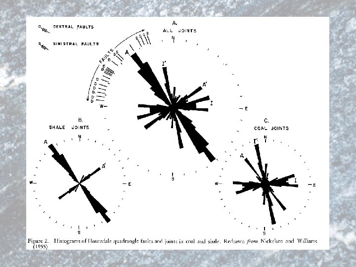
The Rose diagram Fractures from Butler, Chase, and eastern Marion counties. Scale indicates number of sites with joints in 10° intervals; total of 63 sites represented. Major joint sets are numbered (1 -4). Butler County data adapted from Aber (1991).

• How to make a histogram! • We’ve got the following data: {1 1 2 3 3 2 4 5 6 7 4 3 2 3 4 7 8 9 0 0 0 0 1 2 3 3 4 5 5 6 6 4 3 5 2} • Bins…here it is easy: just ten • We count the values… i. e. , how many in bin ‘one’ ‘two’ and so on (there are seven zeroes for example) • We plot the frequencies in the histogram, i. e. , the bins and how many points in each bin. If numbers are not integer, the bins are intervals (i. e. first bin between 0 and one, second bin between one and two and so on).

A Rose Diagram is essentially a histogram: • We bin the hemisphere in an amount of degrees (10 o for example). • Then we count how many joints are in the bin • Normalize to a scale • Plot in the hemisphere

• We’ve got the strikes of the fractures: {15. 4, 20. 1, 18, 12, 15, 16, 77, 76, 73, 74. 5, 73, 16. 2, 17} • Bins: 0 -10, 10 -20, 20 -30…… 350 -360. • Count the points: in the example there are 5 data points in the bin 70 -80, only one data point between 20 -30 and 7 data points between 10 and 20. • Plot in the hemisphere. Each petal length is proportional to the number of data points in the bin.

Sheldon, P. 1912, Some observations and experiments on joint planes: Journal of Geology, Vol. 20, p. 53 -70.

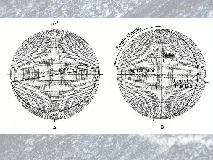
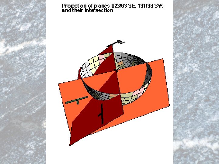
STEREONETS Pole to the plane … when strike & dip has to be represented!

Faults • Faults are fractures along which there has been visible offset by shear displacement (parallel to the fault surface). • Several faults related: Fault zone. • Faults are brittle structures, they are discontinuities in rock, and the primary mechanism for achieving shear displacement at shallow levels. • At deep levels (high P&T) faults grade into shear zones, which are ductile plastic equivalents of faults.

They can be small….

Ok…smaaaaaall 300 µm

At the scale of an outcrop….

Even bigger…

Or f…. huge!!!!

Where is the fault?

Fault Surfaces • A fault surface is the discrete fracture or discontinuity across which rocks do not match up. The term surface is used (rather than plane) to emphasize that faults are rarely truly planar features. • In general, fault surfaces are roughly elliptical, with aspect ratios between 2: 1 to 3: 1. Displacement is maximum at the center of the ellipse and goes to zero at the tip-line-loop, which is like a dislocation in that it separates slipped (faulted) rock from un-slipped rock.

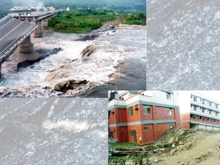
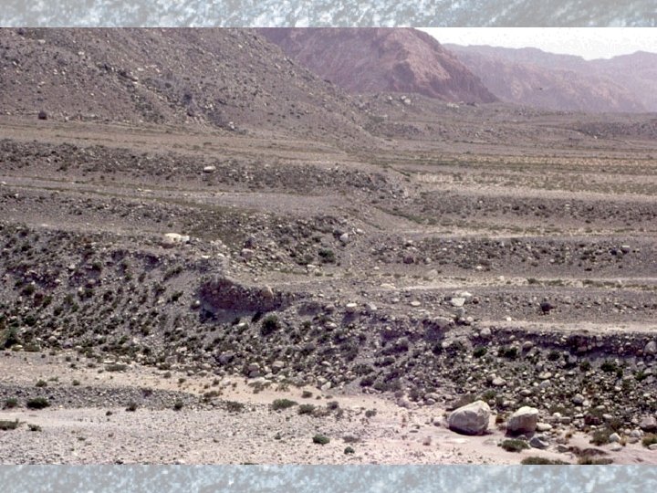
Physical Character of Faults: Scarps • Fault motion produces offset in both natural and man-made objects. • The surface expression of a fault is a fault scarp. • Scarps sometimes do not mark the exact location of a fault, but rather may be modified by erosion, and therefore mark the approximate location of the fault.

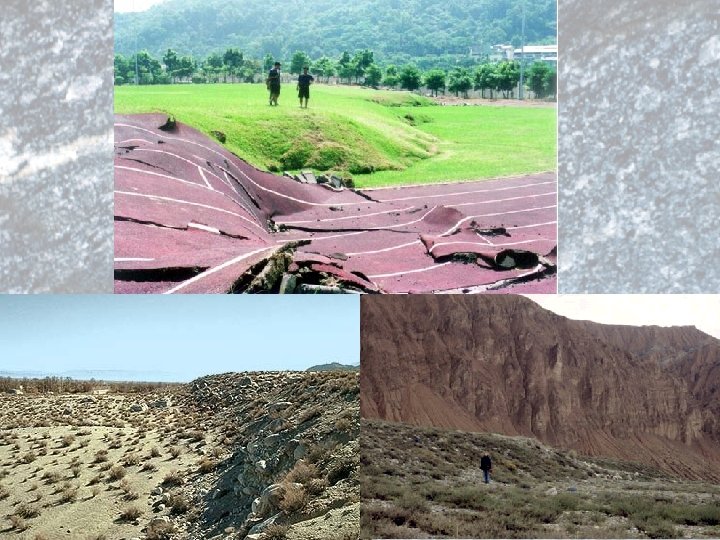
Triangular Facets: eroded fault plane

Triangular Facets: eroded fault plane

Fault Type 1 - Dip-slip faults 1) 2) Terms: Hanging wall and footwall Normal faults (a) Grabens (b) Horsts 3) Reverse faults a) low angle called Thrust faults 4) Oblique-slip faults

Dip-Slip Faults

(Look at the angle) Key Bed

Normal fault (Hanging wall down)

Reverse fault (called “Thrust fault” if shallow angle, < 30º) (Hanging wall up) Younger

Types of Faults - 2 Strike-slip faults Distinctive landforms (linear valleys, chains of lakes, sag ponds, topographic saddles, shutter ridges, offset streams)

San Andreas Fault

Horizontal Movement Along Strike-Slip Fault

Oblique Slip Also seen in Transform Faults such as San Andreas

Miranda convection