
Globally Consistent Range Scan Alignment for Environment Mapping
Globally Consistent Range Scan Alignment for Environment Mapping F. LU ∗ AND E. MILIOS Department of Computer Science, York University, North York, Ontario, Canada eem@cs. yorku. ca
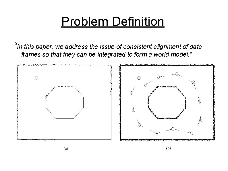
Problem Definition “In this paper, we address the issue of consistent alignment of data frames so that they can be integrated to form a world model. ”
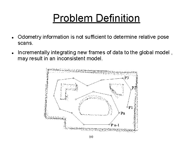
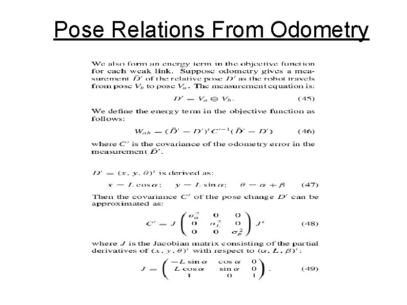
Problem Definition Odometry information is not sufficient to determine relative pose scans. Incrementally integrating new frames of data to the global model , may result in an inconsistent model.
Related Work HILARE project (Chatila and Laumond, 1985). Moutarlier and Chatila, 1989. Durrant-Whyte (1987, 1988 a, 1988 b) Tang and Lee (1992)
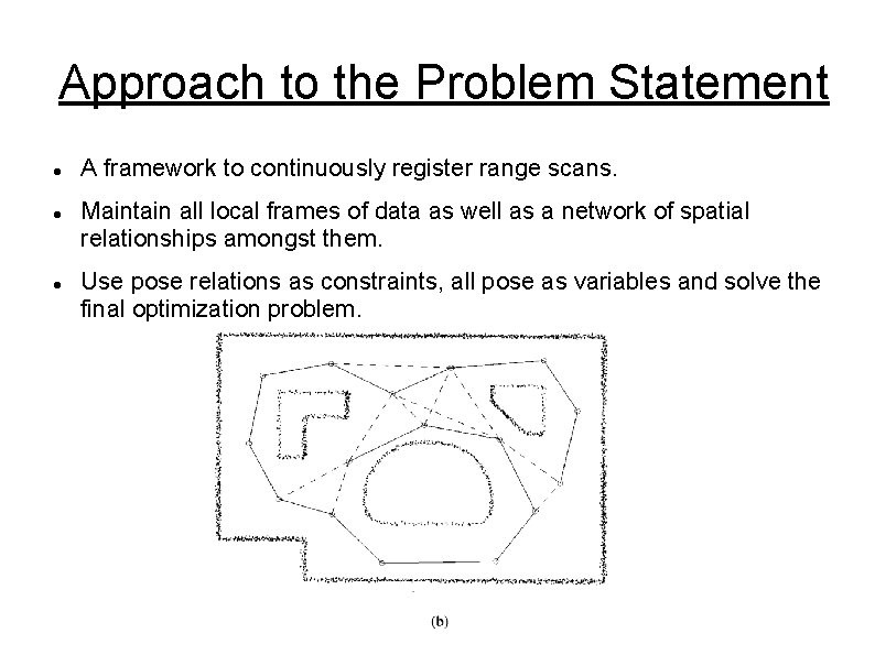
Approach to the Problem Statement A framework to continuously register range scans. Maintain all local frames of data as well as a network of spatial relationships amongst them. Use pose relations as constraints, all pose as variables and solve the final optimization problem.
Deriving Pose Relations Pose relations can be directly obtained from odometry or aligning pairwise scans of points. The corresponding points from the two scans will form a constraint between the two poses. The pose relation is derived from the overlapping potion of the two scans.
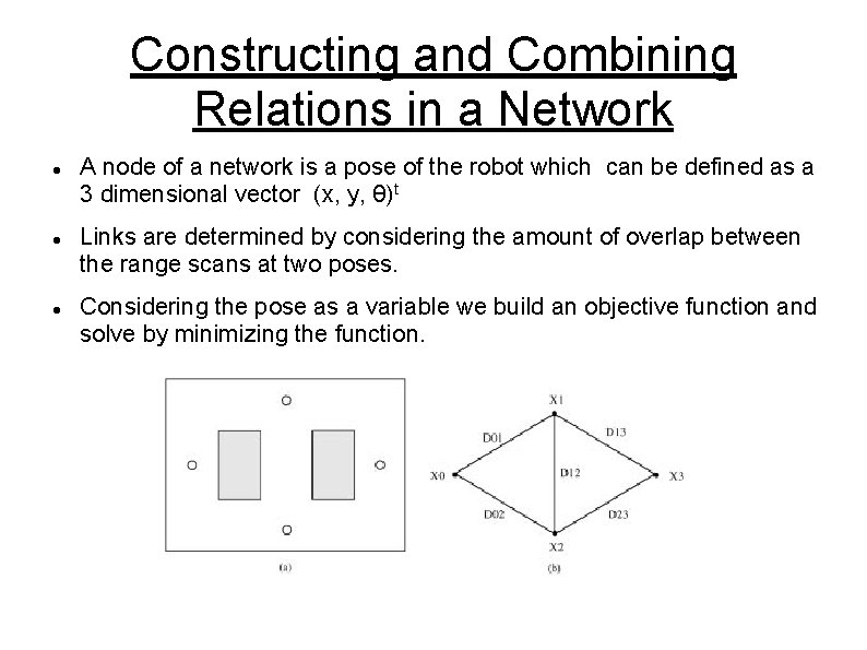
Constructing and Combining Relations in a Network A node of a network is a pose of the robot which can be defined as a 3 dimensional vector (x, y, θ)t Links are determined by considering the amount of overlap between the range scans at two poses. Considering the pose as a variable we build an objective function and solve by minimizing the function.
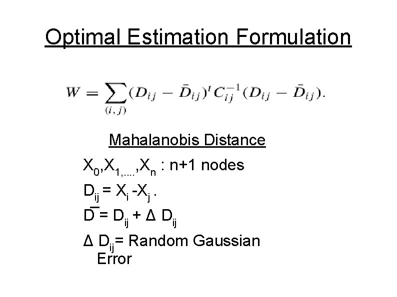
Optimal Estimation Formulation Mahalanobis Distance X 0, X 1, . . , Xn : n+1 nodes Dij = Xi -Xj. D = Dij + Δ Dij= Random Gaussian Error
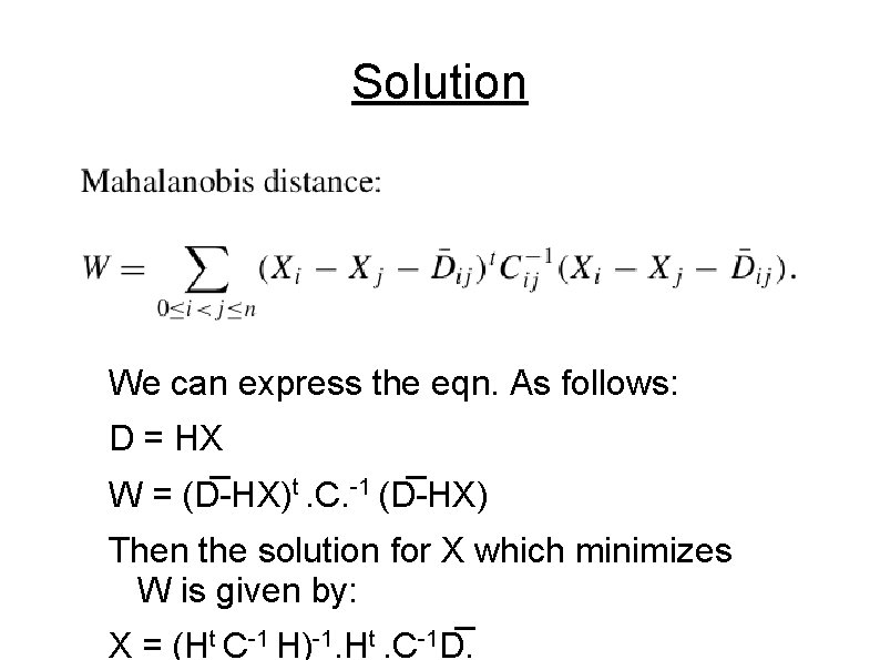
Solution We can express the eqn. As follows: D = HX W = (D -HX)t. C. -1 (D -HX) Then the solution for X which minimizes W is given by: X = (Ht C-1 H)-1. Ht. C-1 D.

Solution Continues. . Denoting Ht. C-1 H by G, and expanding the matrix multiplications we can obtain d*d sub matrices of G as:
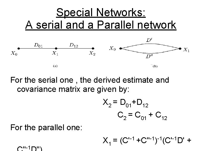
Special Networks: A serial and a Parallel network For the serial one , the derived estimate and covariance matrix are given by: X 2 = D 01+D 12 C 2 = C 01 + C 12 For the parallel one: -1 X 1 = (C'-1 +C''-1)-1(C'-1 D' +

Wheatstone Bridge Network
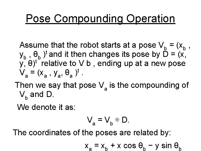
Pose Compounding Operation Assume that the robot starts at a pose Vb = (xb , yb , θb )t and it then changes its pose by D = (x, y, θ)t relative to V b , ending up at a new pose Va = (xa , ya, θa )t. Then we say that pose Va is the compounding of Vb and D. We denote it as: Va = Vb ⊕ D. The coordinates of the poses are related by: xa = xb + x cos θb − y sin θb
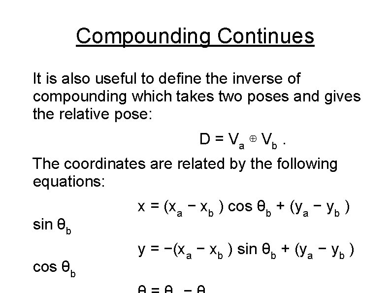
Compounding Continues It is also useful to define the inverse of compounding which takes two poses and gives the relative pose: D = V a ⊕ Vb. The coordinates are related by the following equations: sin θb cos θb x = (xa − xb ) cos θb + (ya − yb ) y = −(xa − xb ) sin θb + (ya − yb )
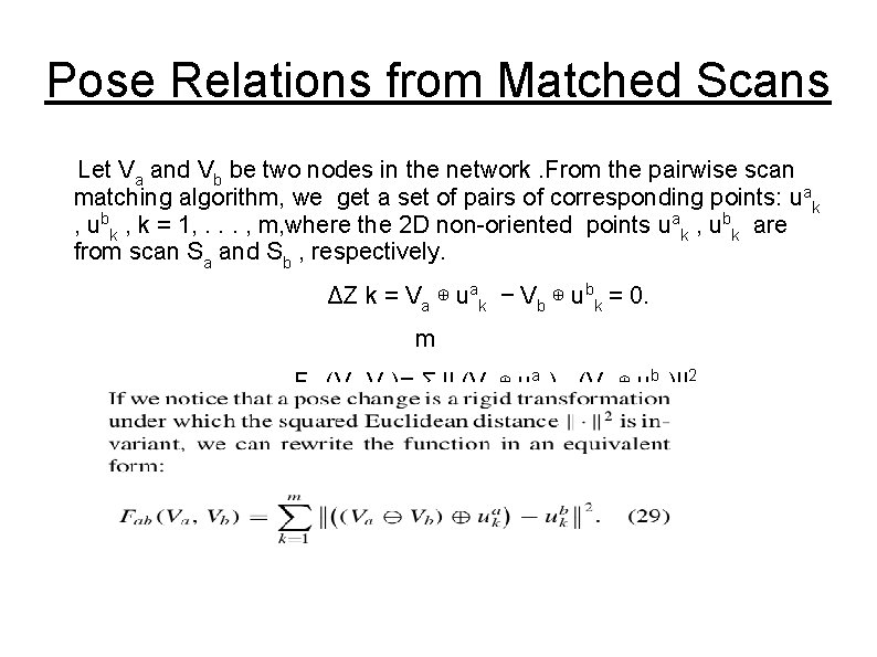
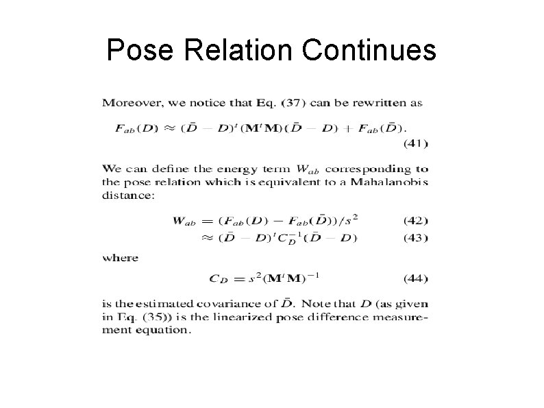
Pose Relations from Matched Scans Let Va and Vb be two nodes in the network. From the pairwise scan matching algorithm, we get a set of pairs of corresponding points: uak , ubk , k = 1, . . . , m, where the 2 D non-oriented points uak , ubk are from scan Sa and Sb , respectively. ΔZ k = Va ⊕ uak − Vb ⊕ ubk = 0. m Fab(Va, Vb)= Σ || (Va ⊕ uak) - (Vb ⊕ ubk)||2 K= 1
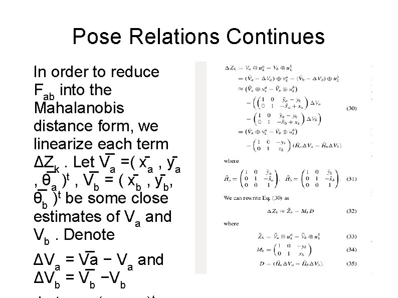
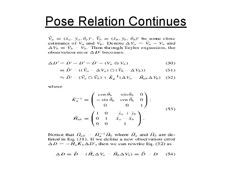
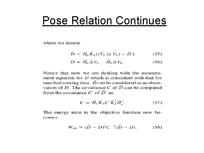
Pose Relations Continues In order to reduce Fab into the Mahalanobis distance form, we linearize each term ΔZk. Let V a =( x a , y a , θ a )t , V b = ( x b , y b, θ b )t be some close estimates of Va and Vb. Denote ΔVa = V a − Va and ΔVb = V b −Vb
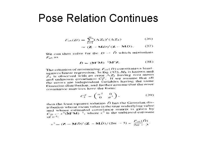
Pose Relation Continues
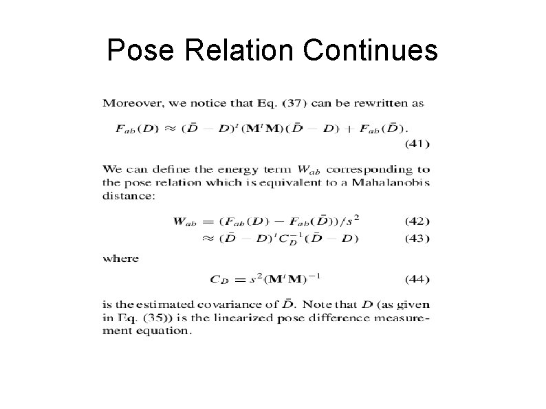
Pose Relation Continues
Pose Relation Continues
Pose Relations From Odometry
Pose Relation Continues
Pose Relation Continues
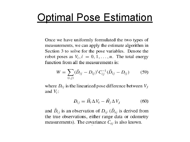
Optimal Pose Estimation
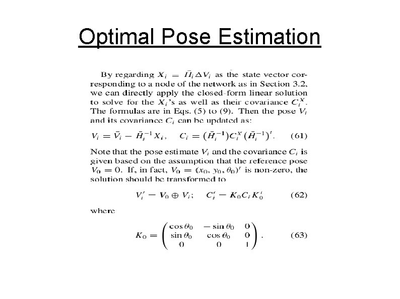
Optimal Pose Estimation
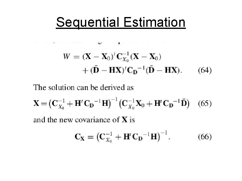
Sequential Estimation
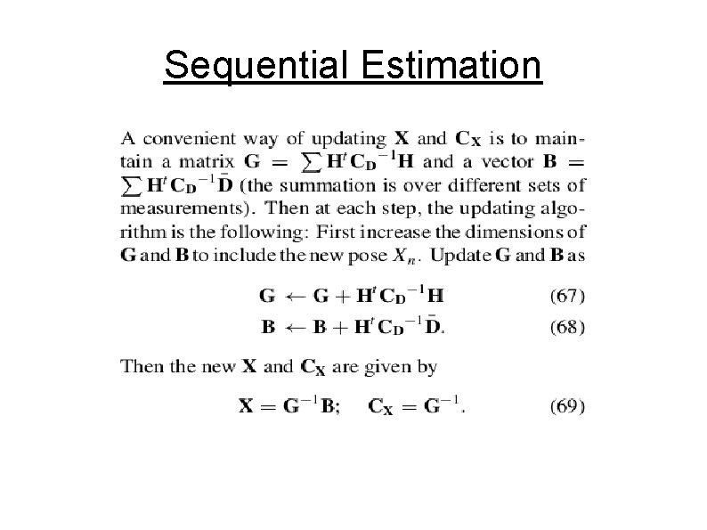
Sequential Estimation
Conclusion In this paper, we formulated the problem of consistent range data registration as one of optimal pose estimation from a network of relations. Although we develop our method for mapping a 2 D environment using 2 D range scans, our formulation is general and it can be applied to the 3 D case as well, by generalizing pose composition an linearization.
- Slides: 27