Global Forecast System GFS What is GFS Global
")
Global Forecast System (GFS)
 is often mislabeled or misunderstood. Global Forecast")
What is GFS? Global Forecast System (GFS) is often mislabeled or misunderstood. Global Forecast System is the full global scale numerical weather prediction system – It includes both the global analysis and forecast components However, the term GFS has also been used to imply that it is the NCEP global spectral model. Therefore, we may use the term GFS to imply both the atmospheric model as well as the whole forecast system
 with transformation")
NCEP Global Spectral model Horizontal Representation • Spectral (spherical harmonic basis functions) with transformation to a Gaussian grid for calculation of nonlinear quantities and physics • Horizontal resolution • > Operational version - T 574 up to 192 hours and T 190 to 384 hours • > Supported resolutions – T 574, T 382, T 254, T 190, T 170, T 126 and T 62

• Initialization – Digital filter initialization with 3 hour window. Time integration scheme: – Leapfrog for nonlinear advection terms – Semi-implicit for gravity waves and zonal advection of vorticity and specific humidity. – Asselin (1972) time filter to control computational mode – Time split physics adjustments with implicit treatment when possible

Vertical Domain • Sigma-Pressure hybrid coordinate system • Terrain following near the lower boundary • Constant pressure surfaces in the stratosphere and beyond • Operationally 64 hybrid layers (15 levels below ~ 800 h. Pa and 24 levels above 100 h. Pa. • 28, 42 and 91 layer options available.

Model Dynamics • Prognostic equations – Primitive equations in hybrid sigma-pressure vertical coordinates for vorticity, divergence, ln(Ps), virtual temperature, and tracers. – Tracers can be specific humidity, ozone mixing ratio and cloud condensate mixing ratio or any other aerosol/dust etc. – Operationally only three tracers.

Vertical Advection Until the last GFS implementation, the vertical advection of tracers were based on ca entered difference scheme This resulted in to the computationally generated negative tracers In the last implementation a positive-definite tracer transport scheme was implemented which minimised the generation of negative tracers. This change was necessary for the newly implemented GSI which is sensitive to the negative water vapor. 7

Vertical Advection of Tracers: previous GFS Scheme Flux form conserves mass Current GFS uses central differencing in space and leap-frog in time. The scheme is not positive definite and may produce negative tracers. 8

Example: Removal of Negative Water Vapor Sources of Negative Water Vapor • Data. Vertical advection • assimilation • Spectral transform • Borrowing by cloud water • SAS Convection _ Ops GFS Data Assimilation Flux-Limited Vertically-Filtered Scheme, central in time Data Assimilation New B: horizontal advection, computed in spectral form with central differencing in space Positive-definite A: vertical advection, computed in finite-difference form with flux-limited positive-definite scheme in space Fanglin Yang et al. , 2009: On the Negative Water Vapor in the NCEP GFS: Sources and Solution. 23 rd Conference on Weather Analysis and Forecasting/19 th Conference on Numerical Weather Prediction, 1 -5 June 2009, Omaha, NE 9
 Van Leer (1974) Limiter, anti -diffusive")
Vertical Advection of Tracers: Flux-Limited Scheme Thuburn (1993) Van Leer (1974) Limiter, anti -diffusive term Special boundary conditions 10
 Van Leer (1974) Limiter, anti -diffusive")
Vertical Advection of Tracers: Flux-Limited Scheme Thuburn (1993) Van Leer (1974) Limiter, anti -diffusive term Special boundary condition 11
 Initial condition Flux-Limited GFS")
Vertical Advection of Tracers: Idealized Case Study wind Upwind (diffusive) Initial condition Flux-Limited GFS Central-in-Space 12

Summary: Negative Water Vapor in the GFS Causes Importance Solutions Vertical Advection 1. Semi-Lagrangian 2. Flux-Limited Positive. Definite Scheme for current Eulerian GFS GSI Analysis Tuning factqmin and factqmax Spectral Transform 1. Semi-Lagrangian GFS: running tracers on grid, no spectral transform 2. Eulerian GFS: no solution yet. Cloud Water Borrowing Limiting the borrowing to available amount of water vapor SAS Mass-Flux Remains to be resolved 13

Horizontal Diffusion • Scale selective 8 th order diffusion of Divergence, vorticity, virtual, temperature, specific humidity, ozone and cloud condensate. • Temperature diffusion in done on quasi-pressure surfaces

Algorithm of the GFS Spectral Model One time step loop is divided into : – Computation of the tendencies of divergence, log of surface pressure and virtual temperature and of the predicted values of the vorticity and moisture (grid) – Semi-implicit time integration – Time filter does not require the predicted variables – Time split physics (transform grid) – Damping to simulate subgrid dissipation – Completion of the time filter

GFS Parallelism Spectral • Spectral fields separated into their real and imaginary parts to remove stride problems in the transforms • Hybrid 1 -D MPI with Open. MP threading – Spectral space 1 -D MPI distributed over zonal wave numbers (l's). Threading used on variables x levels • Cyclic distribution of l's used for load balancing the MPI tasks due to smaller numbers of meridional points per zonal wave number as the wave number increases. For example for 4 MPI tasks the l's would be distributed as 12344321

GFS Parallelism-Grid – Grid space 1 -D MPI distributed over latitudes. Threading used on longitude points. • Cyclic distribution of latitudes used for load balancing the MPI tasks due to smaller number of longitude points per latitude as latitude increases (approaches the poles). For example for 4 MPI tasks the latitudes would be distributed as 12344321 • NGPTC (namelist variable) defines number (block) of longitude points per group (vector length per processor) that each thread will work on

GFS Scalability • 1 -D MPI scales well to 2/3 of the spectral truncation. For T 574 about 400 MPI tasks. • Open. MP threading performs well to 8 threads and still shows decent scalability to 16 threads. • T 574 scales to 400 x 16 = 6400 processors.
 • Nonlocal PBL scheme originally")
Model Physics Planetary Boundary Layer and vertical diffusion (PBL) • Nonlocal PBL scheme originally proposed by Troen and Mahrt (1986) and implemented by Hong and Pan (1996) • First order vertical diffusion scheme • PBL height estimated iteratively from ground up using bulk Richardson number • Diffusivity calculated as a cubic function of height and determined by matching with surface fluxes • Counter-gradient flux parameterization based on the surface fluxes and convective velocity scale. • Recent update – stratocumulus top driven vertical diffusion scheme to enhance diffusion in cloudy regions when CTEI exists • For the nighttime stable PBL, local diffusivity scheme used. • Exponentially decreasing diffusivity for heat and moisture • Constant background diffusivity of 3 m 2/s for momentum

New PBL scheme • Include stratocumulus-top driven turbulence mixing. • Enhance stratocumulus top driven diffusion when the condition for cloud top entrainment instability is met. • Use local diffusion for the nighttime stable PBL. • Background diffusion in inversion layers below 2. 5 km over ocean is reduced by 70% to decrease the erosion of stratocumulus along the costal area. (Moorthi)
")
Diffusion in stable boundary layer MRF PBL Revised model Local diffusion scheme (Louis, 1979) Rbcr=0. 25 l 0 = 150 m for unstable condition 30 m for stable condition * Use local diffusion scheme above PBL for both MRF and new models
 where")
Heat flux MRF PBL Revised model (Simplified after Lock et al. , 2000) where c=0. 2 C=1. 0 (CTEI condition)

Model Physics Sub-grid scale gravity wave drag and mountain blocking

Correction of model bias from sub-grid scale parameterization is an on-going process. Atmospheric flow is significantly influenced by orography, creating lift and frictional forces The unresolved sub-grid scale orography has significant impact on the evolution of the model atmosphere and must be parameterized. Sub-grid scale orography generates vertically propagating gravity waves transferring momentum aloft. Gravity wave Drag, implemented in 1987, and 1997 Mountain Blocking, implemented 2004

• Mountain blocking of wind flow around sub-gridscale orography is a process that retards motion at various model vertical levels near or in the boundary layer. • Flow around the mountain encounters larger frictional forces by being in contact with the mountain surfaces for longer time as well as the interaction of the atmospheric environment and vortex shedding which is shown to occur in numerous observations and tank simulations. • Snyder, et al. , 1985, observed the behavior of flow around or over obstacles and used a dividing streamline to analyze the level where flow goes around a barrier or over it.
 incorporated the dividing streamline into the ECMWF global")
• Lott and Miller (1997) incorporated the dividing streamline into the ECMWF global model, as a function of the stable stratification, where above the dividing streamline, gravity waves are potentially generated and propagate vertically, and below, the flow is expected to go around the barrier with increased friction in low layers.

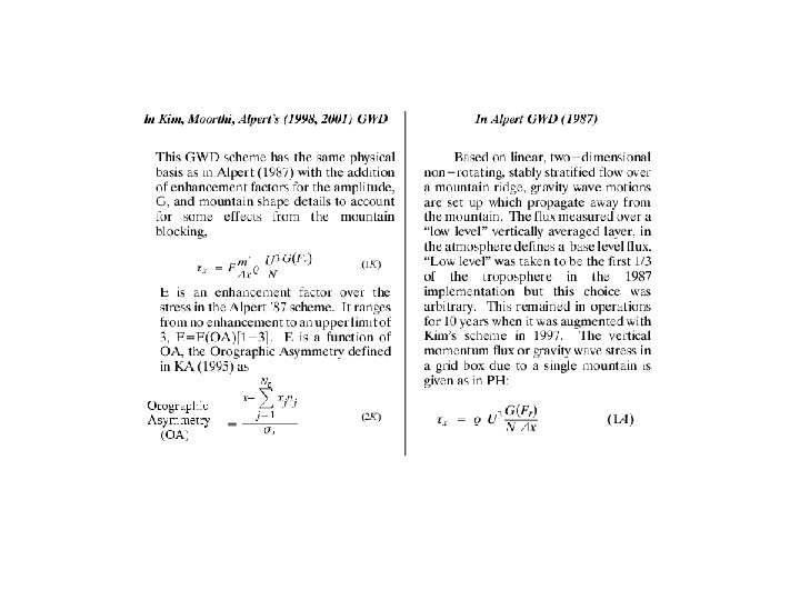
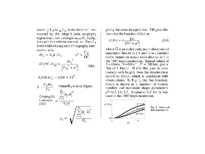
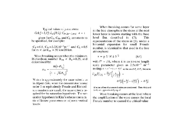
• An augmentation to the gravity wave drag scheme in the NCEP global forecast system (GFS), following the work of Alpert et al. , (1988, 1996) and Kim and Arakawa (1995), is incorporated from the Lott and Miller (1997) scheme with minor changes and including the dividing streamline.

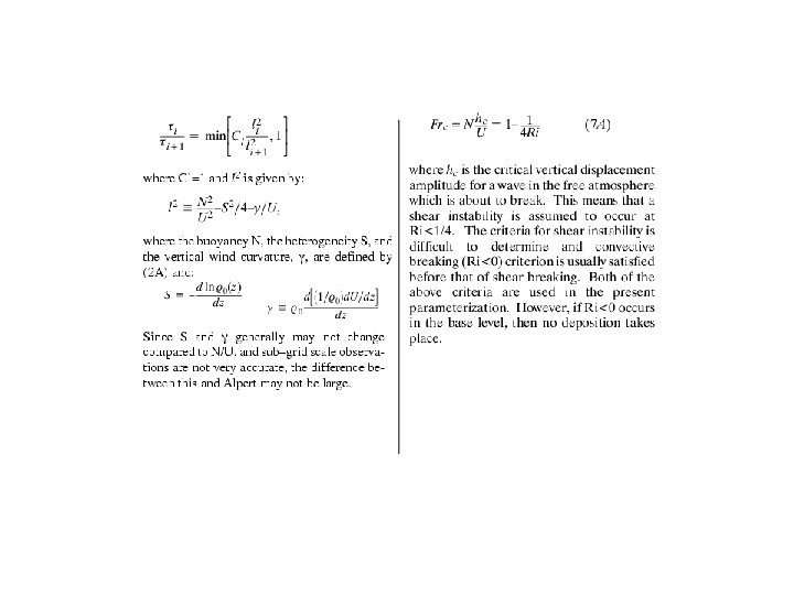
• The idea of a dividing streamline at some level, hd, as in Snyder et al. (1985) and Etling, (1989), dividing air parcels that go over the mountain from those forced around an obstacle is used to parameterize mountain blocking effects. Lott and Miller (1997) incorporated the dividing streamline into the ECMWF global model, as a function of the stable stratification. Above the dividing streamline, gravity waves are potentially generated and propagate vertically. Below, the flow is expected to go around the barrier with increased friction in lower layers
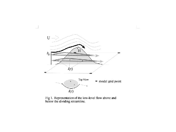

The dividing streamline height, of a sub-grid scale obstacle, can be found from comparing the potential and kinetic energies of up stream large scale wind and sub-grid scale air parcel movements. These can be defined by the wind and stability as measured by N, the Brunt Vaisala frequency. The dividing streamline height, hd, can be found by solving an integral equation for hd: where H is the maximum elevation within the sub-grid scale grid box of the actual orography, h, from the GTOPO 30 dataset of the U. S. Geological Survey.

In the formulation, the actual orography is replaced by an equivalent elliptic mountain with parameters derived from the topographic gradient correlation tensor, Hij: and standard deviation, h'. The model sub-grid scale orography is represented by four parameters, after Baines and Palmer (1990), h', the standard deviation, and , s, , the anisotropy, slope and geographical orientation of the orography form the principal components of Hij, respectively. These parameters will change with changing model resolution.

In each model layer below the dividing streamline a drag from the blocked flow is exerted by the obstacle on the large scale flow and is calculated as in Lott and Miller (1997): where l(z) is the length scale of the effective contact length of the obstacle on the sub grid scale at the height z and constant Cd ~ 1. l(z) = F(z, hd, h‘, g, s, Q, ) Where = Q - , the geographical orientation of the orography minus the low level wind vector direction angle, .
 according to Lott and Miller: (1) (2) (3) Term (1) relates")
The function l(z) according to Lott and Miller: (1) (2) (3) Term (1) relates the eccentricity parameters, a, b, to the sub-grid scale orography parameters, a ~ h‘/s and a/b = and allows the drag coefficient, Cd to vary with the aspect ratio of the obstacle as seen by the incident flow since it is twice as large for flow normal to an elongated obstacle compared to flow around an isotropic obstacle. Term (2) accounts for the width and summing up a number of contributions of elliptic obstacles, and Term (3) takes into account the flow direction in one grid region.

5

Model Physics Shallow convection parameterization • Until July 2010, the shallow convection parameterization was based on Tiedtke (1983) formulation in the form of enhanced vertical diffusion within the cloudy layers. • In july 2010, a new massflux based shallow convection scheme based on Han and pan (2010) was implemented operationally. • Model code still contains the old shallow convection scheme as an option (if you set old_monin=. true. ) with an option to limit the cloud top to below level inverstion when CTEI does not exist.

Updated new mass flux shallow convection scheme • Detrain cloud water from every updraft layer • Convection starting level is defined as the level of maximum moist static energy within PBL • Cloud top is limited to 700 h. Pa. • Entrainment rate is given to be inversely proportional to height and detrainment rate is set to be a constant as entrainment rate at the cloud base. • Mass flux at cloud base is given to be a function of convective boundary layer velocity scale.

Updated new shallow convection scheme • Entrainment rate: Siebesma et al. 2003: ce =0. 3 in this study • Detrainment rate = Entrainment rate at cloud base
 Siebesma et al. (2003, JAS) LES studies")
Siebesma & Cuijpers (1995, JAS) Siebesma et al. (2003, JAS) LES studies

Updated new shallow convection scheme Mass flux at cloud base: Mb=0. 03 w* (Grant, 2001) (Convective boundary layer velocity scale)
 scheme is used operationally")
Model Physics Deep convection parameterization • Simplified Arakawa Schubert (SAS) scheme is used operationally in GFS (Pan and Wu, 1994, based on Arakawa-Schubert (1974) as simplified by Grell (1993)) • Includes saturated downdraft and evaporation of precipitation • One cloud-type per every time step • Until July 2010, random clouds were invoked. • Significant changes to SAS were made during July 2010 implementation which helped reduce excessive grid-scale precipitation occurrences.

Updated deep convection scheme • No random cloud top – single deep cloud assumed • Cloud water is detrained from every cloud layer. • Specified finite entrainment and detrainment rates for heat, moisture, and momentum • Similar to shallow convection scheme, in the subcloud layers, the entrainment rate is inversely proportional to height and the detrainment rate is set to be a constant equal to the cloud base entrainment rate. • Above cloud base, an organized entrainment is added, which is a function of environmental relative humidity.

SAS convection scheme Updraft mass flux CTOP Entrainment DL 1. 0 h LFC SL h 150 mb s Entrainment Downdraft mass flux 1. 0 Detrainment 0. 5 Environmental moist static energy 0. 05
 turb. org. in")
Updated deep convection scheme Organized entrainment (Betchtold et al. , 2008) turb. org. in sub-cloud layers above cloud base
![Updated deep convection scheme Maximum mass flux [currently 0. 1 kg/(m 2 s)] is](http://slidetodoc.com/presentation_image_h2/530f5288b1f39ecdfe25942e0aced732/image-48.jpg "Updated deep convection scheme Maximum mass flux [currently 0. 1 kg/(m 2 s)] is")
Updated deep convection scheme Maximum mass flux [currently 0. 1 kg/(m 2 s)] is defined for the local Courant-Friedrichs-Lewy (CFL) criterion to be satisfied (Jacob and Siebesman, 2003); Then, maximum mass flux is as large as 0. 5 kg/(m 2 s)
 scheme • Include the effect of convection-induced pressure gradient force")
Modification to deep convection(SAS) scheme • Include the effect of convection-induced pressure gradient force in momentum transport (Han and Pan, 2006) c: effect of convection-induced pressure gradient force c=0. 0 in operational SAS c=0. 55 in modified SAS following Zhang and Wu (2003) * Note that this effect also changes updraft and downdraft properties inside the SAS scheme and thus, one should not simply reduce momentum change by convection outside the scheme.
-P(k 1)<150 mb k 2 -k")
Modification in convection trigger Operational pre Jul 2010: P(ks)-P(k 1)<150 mb k 2 -k 1< 2 k 2 LFC k 1 Current operational: 120 mb<P(ks)-P(k 1)<180 mb (proportional to w) P(k 1)-P(k 2) < 25 mb h h* ks h: moist static energy h*: saturation moist static energy

ISCCP Opr. GFS New package

70% reduced backgroud diffusion in inversion layers below 2. 5 km over ocean With original background diffusion
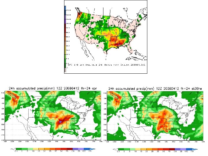
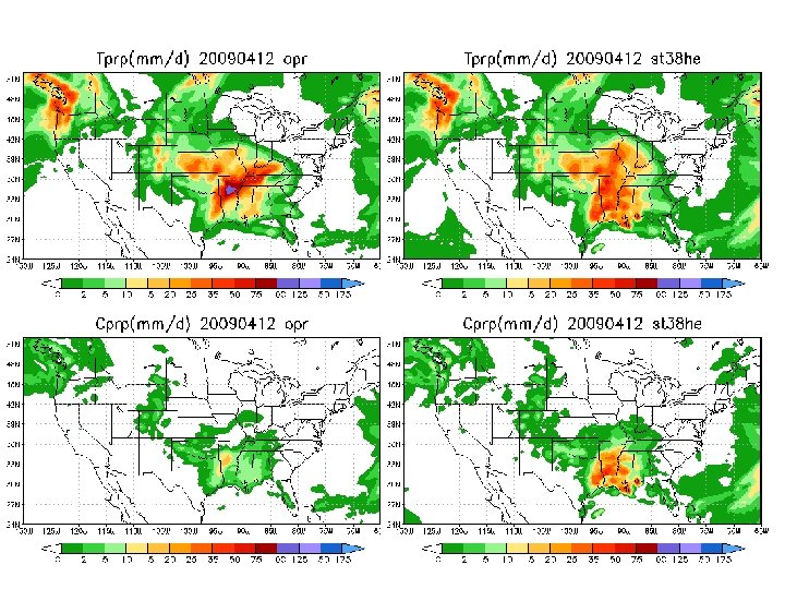

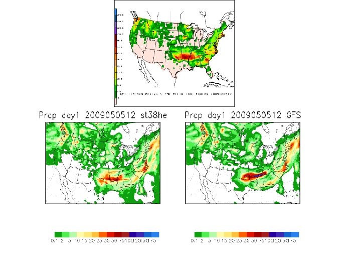
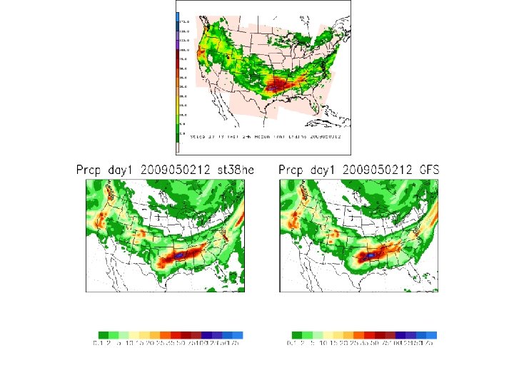
Grid Point Storm 24 h accumulated precip ending 12 UTC 14 July 2009 Observed 48 h GFS Forecast
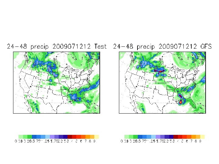

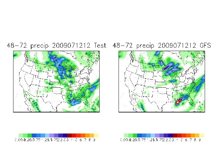
Grid Point Storm 24 h accumulated precip ending 12 UTC 15 July 2009 Observed 72 h GFS Forecast

Model Physics Large-scale condensation and precipitation • The large-scale condensation and precipitation is parameterized following Zhao and Carr (1997) and Sundqvist et al (1989) • This was implemented in GFS along with prognostic cloud condensate in 2001 (Moorthi et al, 2001) • Partitioning between cloud water and ice is made based on the temperature. • Convective cloud detrainment is a source of cloud condensate which can either be precipitated or evaporated through large scale cloud microphysics.

Model Physics Radiation

Unified Radiation Package in NCEP models Features: : Standardized component modules, General plug-in compatible, Simple to use, Easy to upgrade, Efficient, and Flexible in future expansion. • References: • Hou et al. (2011): NCEP Office Note (in preparation) • Hou et al. (2002): NCEP Office Note 441 (ref for clouds, aerosols, and surface albedo processes) • Mlawer and Clough (1998): Shortwave and longwave enhancements in the rapid radiative transfer model, in Proceedings of the 7 th Atmospheric Radiation Measurement (ARM) Science Team Meeting. • Mlawer and Clough (1997): On the extension of rapid radiative transfer model to the shortwave region, in Proceedings of the 6 th Atmospheric Radiation Measurement (ARM) Science Team Meeting. • Mlawer et al. (1997): RRTM, a validated correlated-k model for the longwave, JGR.

Overview Module Structures: Driver Module - prepares atmospheric profiles incl. aerosols, gases, clouds, and surface conditions, etc. Astronomy Module - obtains solar constant, solar zenith angles Aerosol Module - establishes aerosol profiles and optical properties Gas Module - sets up absorbing gases’ profiles (O 3, CO 2, rare gases, etc. ) Cloud module - prepares cloud profiles incl. fraction, ice/water paths, and effective size parameters, etc. Surface module - sets up surface albedo and emissivity SW radiation module - computes SW fluxes and heating rates (contains three parts: parameters, data tables, and main program) LW radiation module - computes LW fluxes and heating rates (contains three parts: parameters, data tables, and main program)

Schematic Radiation Module Structure Driver Module • initialization main driver Aerosol Module initialization clim aerosols GOCART aerosols Derived Type : aerosol_type Surface Module initialization SW albedo LW emissivity Derived Type : sfcalb_type Gases Module Cloud Module initialization solar params ozone prog cld 1 mean coszen co 2 prog cld 2 rare gases diag cld Astronomy Module SW Param Module LW Param Module SW Data Table Module LW Data Table Module SW Main Module LW Main Module initialization sw radiation lw radiation Outputs : total sky heating rates surface fluxes (up/down) toa atms fluxes (up/down) Optional outputs: clear sky heating rates spectral band heating rates fluxes profiles (up/down) surface flux components Outputs : total sky heating rates surface fluxes (up/down) toa atms fluxes (up/down) Optional outputs: clear sky heating rates spectral band heating rates fluxes profiles (up/down)
 • • • ISOL=0:")
Radiation_Astronomy Module Solar constant value : (Cntl parm - ISOL) • • • ISOL=0: use prescribed solar constant (for NWP models) most recent cited value = 1366 w/m 2 (2002) ISOL=1: use prescribed solar constant with 11 -year cycle (for climate models) variation range: 1365. 7 – 1370 w/m 2 obsv data range: 1944 -2006 **tabulated by H. Vandendool
 ICO 2=0: use prescribed")
Radiation_Gases Module CO 2 Distribution : (Cntrol parameter- ICO 2) ICO 2=0: use prescribed global annual mean value (currently set as 380 ppmv) ICO 2=1: use observed global annual mean value ICO 2=2: use observed monthly 2 -d data table in 15° horizontal resolution O 3 Distribution : interactive or climatology Rare Gases : (currently use global mean climatology values) CH 4 - 1. 50 x 10 -6 CO - 1. 50 x 10 -8 CF 22 - 1. 50 x 10 -10 ** all units are in ppmv N 2 O - 0. 31 x 10 -6 CF 11 - 3. 52 x 10 -10 CF 113 - 0. 82 x 10 -10 O 2 - 0. 209 CF 12 - 6. 36 x 10 -10 CCL 4 - 1. 40 x 10 -1

Radiation_Clouds Module Cloud prediction scheme: Prognostic 1: based on Zhao/Moorthi microphysics Prognostic 2: based on Ferrier/Moorthi microphysics Diagnostic : legacy diagnostic scheme based on RH-table lookups Cloud overlapping method: (Cntl parm - IOVR) IOVR = 0: randomly overlapping vertical cloud layers IOVR = 1: maximum-random overlapping vertical cloud layers Sub-grid cloud approximation: (CFS Cntl parm - ISUBC) ISUBC=0: without sub-grid cloud approximation ISUBC=1: with Mc. ICA sub-grid approximation (test mode with prescribed permutation seeds) ISUBC=2: with Mc. ICA sub-grid approximation (random permutation seeds) (This option used in CFSV 2 fore/hindcast model)
 Troposphere: monthly global aerosol climatology in")
Radiation_aerosols Module Aerosol distribution: (Cntl parm - IAER) Troposphere: monthly global aerosol climatology in 15° horizontal resolution (GOCART interactive aerosol scheme under development) Stratosphere: historical recorded volcanic forcing in four zonal mean bands (1850 -2000) IAER – 3 -digit integer flag for volcanic, lw, sw, respectively IAER = 000: no aerosol effect in radiation calculations IAER = 001: sw tropospheric aerosols + background stratospheric IAER = 010: lw tropospheric aerosols + background stratospheric IAER = 011: sw+lw tropospheric aerosols + background stratospheric IAER = 100: sw+lw stratospheric volcanic aerosols only IAER = 101: sw tropospheric aerosol + stratospheric volcanic forcing IAER = 110: lw tropospheric aerosol + stratospheric volcanic forcing IAER = 111: sw+lw tropospheric aerosol + stratospheric volcanic forcing
 IALB = 0: vegetation type")
Radiation_surface Module SW surface albedo: (Cntl parm - IALB) IALB = 0: vegetation type based climatology scheme (monthly data in 1° horizontal resolution) IALB = 1: MODIS retrievals based monthly mean climatology LW surface emissivity: (CFS Cntl parm - IEMS) IEMS = 0: black-body emissivity (=1. 0) IEMS = 1: monthly climatology in 1° horizontal resolution

LW Radiation GFS • • NCEP version: crpnd AER version: No. of bands: No. of g-points: Absorbing gases: Aerosol effect: Cloud overlap: Sub-grid clouds: CFS RRTM 1 RRTM 3 RRTMG_LW_2. 3 RRTMG_LW_4. 82 16 16 140 H 2 O, O 3, CO 2, CH 4, N 2 O, O 2, CO, CFCs yes max-rand no Mc. ICA

SW Radiation GFS • • NCEP version: crpnd AER version: No. of bands: No. of g-points: Absorbing gases: Aerosol effect: Cloud overlap: Sub-grid clouds: CFS RRTM 2 RRTM 3 RRTMG_SW_2. 3 RRTMG_SW_3. 8 14 14 112 --- H 2 O, O 3, CO 2, CH 4, N 2 O, O 2 --yes max-rand no Mc. ICA

Mc. ICA sub-grid cloud approximation • General expression of 1 -D radiation flux calculation: where Fk are spectral corresponding fluxes, and the total number, Κ, depends on different RT schemes Independent column approximation (ICA): where N is the number of total sub-columns in each model grid That leads to a double summation: that is too expensive for most applications! Monte-Carlo independent column approximation (Mc. ICA): In a correlated-k distribution (CKD) approach, if the number of quadrature points (gpoints) are sufficient large and evenly treated, then one may apply the Mc. ICA to reduce computation time. ≈ where k is the number of randomly generated sub-columns Mc. ICA is a complete separation of optical characteristics from RT solver and is proved to be unbiased against ICA (Barker et al. 2002, Barker and Raisanen 2005)

Mc. ICA Distributions of Maximum-Random Overlapped Multi-layer clouds Instance 1 Instance 2

Mc. ICA Distribution of Maximum-Random Overlapping Very Thick Cloud Instance 1 Instance 2

Model Lower Boundary Ocean • SST from the OI analysis at the initial condition time relaxed to climatology with e-folding time of 90 days
")
Model Lower Boundary Land surface model (LSM)

Land modeling at NCEP Shrinivas Moorthi, Michael Ek and the EMC Land-Hydrology Team Environmental Modeling Center (EMC) National Centers for Environmental Prediction (NCEP) 5200 Auth Road, Room 207 Suitland, Maryland 20732 USA National Weather Service (NWS) National Oceanic and Atmospheric Administration (NOAA) April 2011, Indian Institute of Tropical Meteorology, Pune, India

Noah Land Model Connections in NOAA’s NWS Model Production Suite Climate CFS MOM 3 Hurricane GFDL HWRF pled u o C y 2 -Wa Oceans HYCOM Wave. Watch III 1. 7 B Obs/Day Satellites 99. 9% Global Forecast System Global Data Assimilation Regional Data Assimilation North American Ensemble Forecast System GFS, Canadian Global Model NCEPNCAR unified NOAH Land Surface Model Regional NAM Dispersion WRF NMM (including NARR) ARL/HYSPLIT Severe Weather Short-Range Ensemble Forecast WRF: ARW, NMM ETA, RSM WRF NMM/ARW Workstation WRF Air Quality NAM/CMAQ Uncoupled “NLDAS” (drought) Rapid Update for Aviation (ARW-based) For eca st
 & water budgets; 4 soil layers. •")
Noah land-surface model • Surface energy (linearized) & water budgets; 4 soil layers. • Forcing: downward radiation, precip. , temp. , humidity, pressure, wind. • Land states: Tsfc, Tsoil*, soil water* and soil ice, canopy water*, snow depth and snow density. *prognostic • Land data sets: veg. type, green vegetation fraction, soil type, snow-free albedo & maximum snow albedo. • Noah model is coupled with the NCEP Global Forecast System (GFS, medium-range), and Climate Forecast System (CFS, seasonal), & other NCEP models.
 Jan Soil Type (1 -deg, Zobler)")
Land Data Sets Vegetation Type (1 -deg, UMD) Jan Soil Type (1 -deg, Zobler) July Green Vegetation Fraction (monthly, 1/8 -deg, NESDIS/AVHRR) Jan Max. -Snow Albedo (1 -deg, Robinson) July Snow-Free Albedo (seasonal, 1 -deg, Matthews)
: • “Richard’s Equation”; D (soil water diffusivity) and")
Prognostic Equations Soil Moisture ( ): • “Richard’s Equation”; D (soil water diffusivity) and K (hydraulic conductivity), are nonlinear functions of soil moisture and soil type (Cosby et al 1984); F is a source/sink term for precipitation/evapotranspiration. Soil Temperature (T): • CT (thermal heat capacity) and KT soil thermal conductivity; Johansen 1975), are nonlinear functions of soil moisture and soil type. Canopy water (Cw): • P (precipitation) increases Cw, while Ec (canopy water evaporation) decreases Cw.

Atmospheric Energy Budget • Noah land model closes the surface energy budget, & provides surface boundary condition to GFS & CFS. seasonal storage

Surface Energy Budget Rnet = H + LE + G + SPC Rnet = Net radiation = S - S + L - L S = incoming shortwave (provided by atmos. model) S = reflected shortwave (snow-free albedo ( ) provided by atmos. model; modified by Noah model over snow) L = downward longwave (provided by atmos. model) L = emitted longwave = Ts 4 ( =surface emissivity, H LE G SPC = = =Stefan-Boltzmann const. , Ts=surface skin temperature) sensible heat flux latent heat flux (surface evapotranspiration) ground heat flux (subsurface soil heat flux) snow phase-change heat flux (melting snow) • Noah model provides: , L , H, LE, G and SPC.

Hydrological Cycle • Noah land model closes the surface water budget, & provides surface boundary condition to GFS & CFS.

Surface Water Budget S = P – R – E S P R E P-R = = = change in land-surface water precipitation runoff evapotranspiration infiltration of moisture into the soil • S includes changes in soil moisture, snowpack (cold season), and canopy water (dewfall/frostfall and intercepted precipitation, which are small). • Evapotranspiration is a function of surface, soil and vegetation characteristics: canopy water, snow cover/ depth, vegetation type/cover/density & rooting depth/ density, soil type, soil water & ice, surface roughness. • Noah model provides: S, R and E.
 open water")
Potential Evaporation LEp = Rnet-G + cp. Ch. U e + (Penman) open water surface Rnet-G cp Ch U e = = = = slope of saturation vapor pressure curve net radiation air density specific heat surface-layer turbulent exchange coefficient wind speed atmos. vapor pressure deficit (humidity) psychrometric constant, fct(pressure)
 Canopy Water")
Surface Latent Heat Flux LE = LEc + LEt + LEd (Evapotranspiration) Canopy Water Evap. (LEc) canopy water canopy Transpiration (LEt) Bare Soil Evaporation (LEd) soil LEc = function(canopy water %saturation) & LEp LEt = function(Jarvis-Stewart “big-leaf” canopy conductance with vegetation parameters for S , atmos. temp. , e & soil moisture avail. , ) & LEp LEd = fct(soil type, near-surface soil %sat. ) & LEp
 < LE (deep snow) Sublimation (LEsnow)")
Latent Heat Flux over Snow LE (shallow snow) < LE (deep snow) Sublimation (LEsnow) LEsnow = LEp snowpack LEns < LEp LEns = 0 soil Shallow/Patchy Snowcover<1 Deep snow Snowcover=1 • LEns = “non-snow” evaporation (evapotranspiration terms). • 100% snowcover a function of vegetation type, i. e. shallower for grass & crops, deeper forests. • Soil ice = fct(soil type, soil temp. , soil moisture).
 (from canopy/soil snowpack surface) canopy")
Surface Sensible Heat Flux H = cp. Ch. U(Tsfc-Tair) (from canopy/soil snowpack surface) canopy bare soil snowpack soil , cp Ch U Tsfc-Tair = = air density, specific heat surface-layer turbulent exchange coeff. wind speed surface-air temperature difference • “effective” Tsfc for canopy, bare soil, snowpack.
 Heat Flux G = (KT/ z)(Tsfc-Tsoil) (to canopy/soil/snowpack surface) canopy bare")
Ground (Subsurface Soil) Heat Flux G = (KT/ z)(Tsfc-Tsoil) (to canopy/soil/snowpack surface) canopy bare soil snowpack soil KT = soil thermal conductivity (function of soil type: larger for moister soil, larger for clay soil; reduced through canopy, reduced through snowpack) z = upper soil layer thickness Tsfc-Tsoil = surface-upper soil layer temp. difference • “effective” Tsfc for canopy, bare soil, snowpack.

Model Lower Boundary seaice

SEA ICE Model in GFS Xingren Wu EMC/NCEP and IMSG 1/4/2022 Shrinivas Moorthi 95

NSIDC Arctic sea ice hits record low in 2007 9/16/2007 1/4/2022 Shrinivas Moorthi 96

Outline • Sea Ice in the Weather and Climate System • Sea Ice in the NCEP Forecast System - Analysis/Assimilation - Forecast: GFS, CFS • Sea Ice in the CFS Reanalysis 1/4/2022 Shrinivas Moorthi 97

Sea Ice Sea ice is a thin skin of frozen water covering the polar oceans. It is a highly variable feature of the earth’s surface. Greece Ice Melt Pond 1/4/2022 Pancake Ice Nilas & Leads First-Year Ice Snow-Ice Shrinivas Moorthi Multi-Year Ice Rafting 98

Sea ice affects climate and weather related processes Ø Sea ice amplifies any change of climate due to its “positive feedback” (coupled climate model concern): Sea ice is white and reflects solar radiation back to space. More sea ice cools the Earth, less of it warms the Earth. A cooler Earth means more sea ice and vice versa. Ø Sea ice restricts the exchange of heat/water between the air and ocean (NWP concern) ØSea ice modifies air/sea momentum transfer, ocean fresh water balance and ocean circulation: The formation of sea ice injects salt into the ocean which makes the water heavier and causes it to flow downwards to the deep waters and drive a massive ocean circulation 1/4/2022 Shrinivas Moorthi 99

Issues related to sea ice forecast v Data assimilation v Initial conditions v Sea ice models and coupling 1/4/2022 Shrinivas Moorthi 100

Data assimilation issues ü Sea ice concentration data are available but velocity data lack to real time § Lack of sea ice and snow thickness data Initial condition issues ü Sea ice concentration data are available but velocity data lack to real time § Sea ice and snow thickness data are based on model spin-up values or climatology 1/4/2022 Shrinivas Moorthi 101

Sea ice model and coupling issues q q 1/4/2022 Ice thermodynamics Ice model coupling to the atmosphere Ice model coupling to the ocean Shrinivas Moorthi 102

NCEP Sea Ice Analysis Algorithm • 5 minutes latitude-longitude grid from the 85 GHz SSMI information based on NASA Team Algorithm • Half degrees version of the product is used in GFS (as initial condition). Courtesy: Robert Grumbine 1/4/2022 Shrinivas Moorthi 103

Ice Model: Thermodynamics Based on the principle of the conservation of energy, determine: • Ice formation • Ice growth • Ice melting • Ice temperature structure 1/4/2022 Shrinivas Moorthi 104

Sea Ice in the NCEP Global Forecast System • A three-layer thermodynamic sea ice model was embedded into GFS (May 2005). • It predicts sea ice/snow thickness, the surface temperature and ice temperature structure. • In each model grid box, the heat and moisture fluxes and albedo are treated separately for ice and open water. 1/4/2022 Shrinivas Moorthi 105
 Atmospheric model Ice Fraction Ice/Snow Thickness")
Sea Ice in the NCEP GFS (cont. ) Atmospheric model Ice Fraction Ice/Snow Thickness Ice Temperature surface Temperature SW LW Turbulent Snow Heat Flux Rate Ice/Snow Thickness 3 -layer thermodynamics Ice model Salinity Oceanic Heat Flux Ice Fraction Ice Temperature Fresh Water Surface Temperature Ocean model 1/4/2022 Shrinivas Moorthi 106
- Slides: 106