Global energy strategies with low temperature rises An

Global energy strategies with low temperature rises An exploration of energy strategies giving a mean surface temperature rise of less than 2 degrees by 2100, as required by the Paris Agreement, using the DECC Global Calculator Rutherford Appleton Laboratory lecture 24 th November 2016. Jef Ongena Laboratory for Plasma Physics, Royal Military Academy, Brussels, Belgium Chair of the European Physical Society Energy Group Christopher Watson Merton College, Oxford University, UK Chair of the British Pugwash Group

Global Energy Strategies with low temperature rises Did the 193 countries which have signed the United Nations Paris Agreement on Climate Change (COP 21) really know what they meant? Jef Ongena Laboratory for Plasma Physics, Royal Military Academy, Brussels, Belgium Chair of the European Physical Society Energy Group Christopher Watson Merton College, Oxford University, UK Chair of the British Pugwash Group The authors acknowledge with gratitude the influence of the late Prof David Mac. Kay and members of the European Physical Society Energy Group and British Pugwash on the work reported here.

Climate change and global mitigation strategies • Why we have chosen to present this subject to this audience – Need for expertise spanning natural science, engineering, economics and politics/diplomacy – all well represented here. – For a solution to the problem to be valid, the numbers have to add up. – To sustain momentum, we must make demonstrable progress by 2030 – If our generation fails to solve the problem, the consequences for the next generation could be dire. • What progress has our generation made/failed to make? – We have developed a number of potentially relevant energy supply systems, but all have potential limitations or show-stoppers. – Fossil fuels have to be phased out fast, and renewables are intermittent – Our energy end-use solutions are mostly inefficient & need optimising – We are very resistant to changing our lifestyles eg transport, food – Our generation has been slow to recognise the urgency of the problem

Legal status of the Paris Agreement • One year ago, mankind took a genuinely global step to tackle the problem • On 12 December 2015 the 195 Participant Countries meeting in Paris adopted by consensus the United Nations COP 21 Climate Change Agreement • The Agreement was opened for signature on 22 April 2016, and by now 197 Parties to the Convention had signed the Agreement (ie all but 4 of the UN members) and 100 Parties have ratified it (the UK has not yet done so, but has promised to ratify by the end of 2016). So it has recently entered into force. • Each signatory is expected to propose its ‘Nationally-determined contribution’ to the agreed global emissions target, and to report/revise its achievement quinquennially. • But how many of its signatories really understood what it meant?

What is missing from the Paris Agreement? The Agreement lacks: • Baseline data defining the meaning of “pre-industrial levels” • A timetable for reaching stability at a rise level “well below 2 0 C” • A list of the relevant Greenhouse Gases (GHGs) • A procedure for estimating future temperature rises from cumulative GHG emissions • Sufficient clarity in its distinction between the obligations of ‘developed’ and ‘developing’ nations The Conference of the Parties (COP) (and the Ad Hoc Working Group set up by it) need to have rules of procedure governing the process by which they aggregate “Nationally Determined Contributions(NDCs)’’ submitted by the Parties into a “synthesis report”, so that they can then advise the Parties on how their NDCs need modification to enable aggregated emissions to meet the Paris temperature target. The whole process needs to have a sufficiently strong scientific and technological input This paper, presented by members of the European Physical Society Energy Group, and of British Pugwash, seeks to make a contribution to this input.

Some significant international inputs to the subject • • • • The Intergovernmental Panel on Climate Change (IPCC): reports 1990 -2014 The UK Energy Policy Review 1992 The Stern review on the economics of climate change 2006 UK White papers on Nuclear Power and the Climate Change Bill (2008) The UK Department of Energy & Climate Change (DECC) ‘Pathways to 2050’ – a public domain software package enabling the user to design UK energy pathways The EU Treaty of Lisbon (2009) Energiewende: “Energy Concept for an Environmentally Sound, Reliable and Affordable Energy Supply” published by the German Government in Sept 2010 The EU Energy Road Map 2050 (2011) British Pugwash ‘Pathways to 2050’: three possible UK energy strategies Feb 2013 The EU Policy Framework for Climate & Energy for 2020 -2030 (Jan 2014) The position of the Energy Group of the European Physical Society: Nature 2015 “The DECC Global Calculator”: a public domain software package enabling the user to design global energy pathways. This package was designed by an international team led by the UK DECC, and is the basis of the present paper. “Climate Change and the DECC Global Calculator”: a user guide made available on the British Pugwash website in 2015, giving examples of High Nuclear, High Renewable and Intermediate Pathways

Commentary on the story so far • • • The IPCC has given vital ongoing leadership on the underlying science, and on the evidence that global warming is a reality that needs urgent attention. The UK has given valuable leadership by providing software tools that generate numbers to underpin valid global energy policy options. Sadly, it has not itself managed to sustain any energy policy for long enough to enjoy the benefits. Germany has over-reacted to Fukushima, and has sustained its Energiewende policy to the neglect of its implications for the national economy & energy costs. It is making a very large investment in renewables, but well before solutions on the required scale and cost have become available to tackle renewable intermittency. The EU needs to make more realistic economic and technical assessments of its energy policy. For example, in the past 20 years Germany has spent ~€ 1012 on renewables with nearly no benefit in total CO 2 output. No European country is currently putting large resources into Carbon Capture & Storage. The DECC Global Calculator has become available at exactly the right time to explore pathways which can allow the world to meet the Paris targets. Unfortunately it is not quite sufficiently user-friendly to make such explorations easy for the lay user. This paper seeks to assist in this process.

The DECC Global Calculator I • The DECC Global Calculator is a public-domain software package, which was developed by an international consortium led by the UK Department of Energy & Climate Change (DECC), and was put on their website in 2013. Its objective is to give users a tool to devise strategies for mitigating anthropogenic climate change, so that they can provide guidance to policymakers on feasible options. • The user is invited to specify values for about 50 parameters (the so-called ‘levers’) which define a global energy supply and demand system. The software then computes its global emissions of GHGs on an annual basis, starting from preindustrial times, and going up to 2050, using the best available scientific and technical data, and then extrapolates these up to 2100 using a well-defined, but inevitably less precise algorithm. • The package then uses the most recent guidance from the IPCC to forecast the probable resulting global average surface temperature rise from pre-industrial times up to 2100.

The DECC Global Calculator II • The DECC package also reports the lever values proposed by 26 expert organisations, each suggesting one possible ‘pathway’ which the international community might take. In a previous paper (see the last bullet of slide 5) we analysed the outputs provided by the Global Calculator for each of the 26 ‘example’ pathways, and tabulated the main components of the primary energy supply, final energy demand, emissions and temperature rise for each pathway. We found that very few of these example pathways in fact lead to a temperature rise by 2100 of less than 20 C. Over half exceeded 2. 3 0 C and 10 exceeded 2. 5 0 C. • To see whether the Calculator could give Paris-compatible results, we took three of the DECC example pathways (WNA Allegro, CLIMACT and ICEPT) as starting points for our exploration of the parameter space. These pathways represent three broadly different global energy strategies – ‘High Nuclear’, ‘High Renewable’ and ‘Intermediate’ (the last of which also includes a reasonably large amount of Carbon Capture & Storage). We then attempted to ‘fine-tune’ each of these baseline pathways, varying one (or at most two) lever values at a time. In each case, we selected levers which seemed to offer a promising reduction in its contribution to cumulative emissions for that pathway.

The DECC Global Calculator III • The Global Calculator is supplied in two rather different, but mutually compatible, forms: – The spreadsheet version, consisting of some 40 linked Excel spreadsheets – The webtool version, a relatively user-friendly interactive package, with the same lever inputs, some numerical outputs and some helpful graphics Both versions use essentially the same algorithms to make the calculations • The spreadsheet version incorporates a lot of information about the mechanisms leading to the emissions of Greenhouse Gases: – It tracks the actual historic emissions of four key gases – CO 2, CH 4, N 2 O and SO 2 – It calculates the emissions resulting from the user’s pathway choices for each quinquennium up to 2050, taking account of foreseen improvements in industrial practices (see notes in the spreadsheet entitled ‘Outputs-Emissions’) – It estimates the further emissions up to 2100 by extrapolation from those up to 2050, and uses these to estimate the cumulative GHG gas emissions to 2100, taking account of foreseen CCS and agricultural sequestration – All these figures are broken down by the 8 IPCC-defined source sectors, and by the gas concerned, and expressed in Gt of CO 2 e (see ‘Outputs-Emissions’ l 45 -70)

The DECC Global Calculator IV • The final step in the calculation is to convert figures for cumulative GHG emissions into estimates of temperature rise. This is based on the latest IPCC findings, drawing on results obtained from world-wide Global Climatology computer models. • The IPCC has assembled outputs from runs of over 100 such models, in each case taking the same start date and actual/forecast emissions data, and has plotted these up to 2050 in what has come to be called a ’spaghetti diagram’ (see 5 th assessment report page 87) • A statistical analysis has been made of such diagrams, giving curves for an estimated ‘mean value’ of the temperature rise per year and curves giving one standard deviation for those estimates • Analytic approximations to these curves have been fed into the Calculator, and these have been modified to allow for other forcings (halocarbons, VOCs, black carbon, etc) and other uncertainties (see Spreadsheet User Guide pp 40 -47 and the Spreadsheet tab labelled ‘Climate Impacts’). • The output from its calculations of temperature rise is presented in the webtool version of the Calculator as a thermometer showing a band of possible rises in 2100, with numerical values indicating the probable range. In this paper we take the mid-point of this range as the most likely value.

Outputs of forecasts commissioned by IPCC from a range of independent climate models using specified emissions from 2005 to 2050 • EE The heavy black line summarises historical observations: the ensemble of coloured lines represent forecasts by individual climate models, all set to start at 2005. (Source IPCC 5 th Assessment Report WG 1 AR 5 page 87)

Commentary • • The IPCC, and the Global Calculator which draws on it, show a very proper respect for the scientific uncertainties surrounding industrial and climatological predictions extending up to 2100. The world will shortly have to take decisions about the relative sizes of the nuclear, renewable and CCS components of both the global and the various national energy mixes. All three components are threatened by potential ‘show-stoppers’ – technical issues which might make elements of those policy decisions technically or economically non-viable. Even if they are broadly viable, future technical developments may influence their emissions. The link between emissions and temperature rise depends on Global Climatology, which is still a very inexact science, and its imprecision increases with the duration of its forecast. Nevertheless the direction of the trend is clear, and its magnitude is the best evidence that policy-makers currently have. The Global Calculator correctly (and helpfully) emphasises the uncertainties in its predicted temperature rises. The connection between the global average surface temperature rise, and more local events such as hurricanes, polar icecap melting, avalanches, flooding, droughts etc is still conjectural, but evidence of the connection is becoming stronger. Other longer-term effects, such as disruption of agriculture, loss of eco-systems and species, mass movements of populations, wars over loss of resources such as water supply and food etc, become progressively more likely as ΔT increases beyond 2 0 C.

Exploration of the Global Calculator parameter space I The three ‘representative pathways’ chosen as baselines for our exploration (‘High Nuclear’ (HN), ‘High Renewable’ (HN), and ‘Intermediate’ (Int)) all start from the same energy mix in 2011 but have very different ultimate pathways. To get energy figures in GWav, multiply EJ/y by 31. 7 • Primary Energy Supply EJ/y High Nuclear Baseline Date 2020 2025 2030 2035 2040 2045 2050 Nuclear fission Solar, wind, wave, tide High Renewables Baseline 2015 2020 2025 2030 2035 2040 2045 2050 Intermediate Baseline 2015 2020 2025 2030 2035 2040 2045 2050 38 48 58 75 90 109 131 30 31 30 27 27 26 30 33 36 38 42 44 47 49 9 14 28 41 60 91 117 3 7 11 19 26 38 58 74 3 8 14 26 38 57 88 112 Geothermal, hydro, heat 31 34 40 50 58 71 81 27 31 35 41 51 61 76 86 27 31 35 41 51 59 72 82 Bioenergy and waste 56 58 63 66 67 71 72 55 54 52 52 52 55 60 67 55 55 56 59 65 75 87 102 484 477 448 406 361 292 241 473 449 432 399 353 305 236 186 473 482 485 466 432 390 327 275 617 633 637 636 634 642 589 572 560 537 511 486 456 440 588 610 625 630 628 626 619 621 Coal, oil, gas, peat Total CCS on fossil power (GW) 1487 16 988 Unabated fossil power (GW) 0 1782 1643 Emissions (Gt in the year) G 1 Fuel Combustion & Fugitives 15 10 36 36 34 30 24 18 11 6 2 3 3 2 2 2 8 8 6 6 7 7 0 0 5 0 0 -1 2 2 1 1 1 27 23 52 47 45 40 35 28 36 37 35 31 26 22 G. 2 Industrial Processes 3 3 2 2 2 G. 4 Agriculture 6 6 7 7 7 8 G. 5 Land Use and Forestry 5 1 1 1 2 2 2 52 48 47 43 39 34 Waste Total – – – – 36 37 36 34 30 25 19 13 2 3 3 3 3 8 8 6 6 6 7 7 7 -1 -1 5 1 0 0 -1 -3 -5 -6 1 1 1 2 2 2 1 1 21 15 52 48 47 44 40 33 26 19 HN is moving towards an even higher nuclear component but is constrained by its chosen rate of build HR has no new nuclear build but continues to operate existing nuclear plant Int has a relatively slow rate of new nuclear build, but a rather stronger growth in bioenergy All three have broadly similar ‘conventional’ renewable components, constrained by the intermittency problem HN applies CCS to all fossil power, HR has almost none, Int applies it to about half fossil fuel by 2050 Emissions are initially dominated by power generation & other fuel use, but are then closely followed by agriculture, land use etc. By 2050, the move towards a low-carbon economy makes the latter relatively more important. Note that emissions from transport, heating etc are counted against the primary fuel from which they derive.

Sankey diagram for HN baseline These diagrams illustrate the complexity of the energy flow from source to end use, and quantify the role of electrification and energy losses between source and end-use. Similar diagrams for the other two baseline pathways are appended Note that to ensure that the width of the energy flow line is proportional to the actual flow, all primary energies are show in EJ appropriate to that flow - eg as thermal energy in the case of nuclear energy

Exploration of the Global Calculator parameter space II In our early attempts to ‘fine-tune’ our three representative pathways, we focused on levers which affected emissions deriving from combustion of primary fuels. These attempts were mostly rather unsuccessful – changes in individual lever values frequently had unintended consequences, and they did not in general greatly decrease the value of ΔT In our recent work, we have therefore focused on variations in the values of lever in the range 33 to 48 – ie levers which affect agriculture and land use. This has proved much more rewarding: • • Variations explored up to 24/11/16 Lever no(s) and significance HN Baseline (High Nuclear) Variation Baseline HR Baseline (High Renewables) Int Baseline (Intermediate) Cumulative CO 2 e to Estimated 2100 (Gt) mean ΔT Variation 2100 (Gt) mean ΔT 3003 2. 45 2882 2. 15 Variation Cumulative CO 2 e to Estimated 2100 (Gt) mean ΔT 2768 2. 1 Var 1 Lever 33 calorie consumption 2. 0 > 3. 5 2747 2. 3 3. 0 > 3. 5 2837 2. 15 2. 0 > 3. 5 2613 2 Var 2 Levers 34&35 Meat consumption/type 2, 3> 3, 3 2508 2. 15 3, 3> 3, 3 2882 2. 15 2, 3> 3, 3 2787 2. 1 Var 5 Levers 34&35 Meat consumption/type 2, 3>3. 5, 3. 5 1638 1. 55 3, 3>3. 5, 3. 5 1913 1. 6 2, 3>3. 5, 3. 5 1941 1. 6 Var 3 Lever 36 Crop yields 1. 7>3. 0 2483 2. 2 2>3 2710 2. 1 1. 7>3. 0 2616 2. 05 Var 6 Lever 36 Crop yields 1. 7>3. 5 2405 2. 2 2>3. 5 2600 2. 05 1. 7>3. 5 2514 1. 95 Var 4 Levers 38, 39 Livestock yields 2, 3>3, 3 2643 2. 3 2, 2>3, 3 2555 2. 05 2, 3>3, 3 2500 2 Var 7 Levers 38, 39 Livestock yields 2, 3>3. 5, 3. 5 2596 2. 35 2, 2>3. 5, 3. 5 2361 2 2, 3>3. 5, 3. 5 2342 1. 95 Var 8 Levers 36, 42 Surplus land use 1. 7, 2. 6> 3. 5, 3 2453 2. 2 2, 1. 3> 3. 5, 3 2992 2. 2 1. 7, 2. 6> 3. 5, 3 2697 2. 1 Var 9 Levers 40, 41 Bioenergy yields 3, 3> 3. 5, 3. 5 2966 2. 45 2, 2> 3. 5, 3. 5 2724 2. 1 3, 3> 3. 5, 3. 5 2612 2. 05 Var 10 Lever 48 Wastes & residues 1. 5 > 3. 0 2498 2. 05 2> 3. 0 2708 2 1. 5 > 3. 0 2614 1. 95

Exploration of the Global Calculator parameter space III • Commentary • None of the baseline ΔT values quite meet the Paris target: however they are sufficiently close to make it worth trying to fine-tune these pathways. • The three baseline ΔT values are not equal: the HN value is significantly higher. This reflects the fact that ‘decarbonisation’ ie the decline in fuel combustion emissions occurs more slowly than in the other two pathways. • All the exploratory variations shown produce strong reductions in ΔT: these are particularly marked where the revised lever value is 3. 5, though in some cases (eg lever 48) even a revised value of 3. 0 is sufficient. • The strongest reduction in ΔT results when levers 34 & 35 are increased to 3. 5 – in this case, for all three baselines the value achieved is ~ 1. 6 • The precise values of ΔT found are probably not statistically significant – all values below about 2. 2 can be regarded as close to the Paris target. • Each of the exploratory variation related to one, or at most two, of the levers: there is clearly scope for further fine-tuning by making simultaneous variations of more lever values, perhaps by smaller amounts. • Some caveats on these findings are discussed in the following two slides.

Exploration of the Global Calculator parameter space IV • Caveats on the level values selected for variations 1 -10 • All the lever values selected lie in the range 3 to 3. 5 This is because the starting values in the baseline pathways were mostly ≥ 2. 0. This is hardly surprising: their designers were attempting to achieve Paris-compliance. The upper limit reflects the fact that the Calculator has some difficulty in handling values in the range 3. 6 -3. 9: its algorithm for urls fails in this range. • The Calculator’s guidance on the use of high values for levers is: – A value of 3 represents a choice of abatement effort which is very ambitious but achievable – A value of 4 is extraordinarily ambitious and extreme: only a minority would think it possible • Among the 26 example pathways, only two make any use of the value 4, and the average lever value set is about 2. 1, with only occasional settings above 3. So our variations in the range 3 to 3. 5 should be regarded as exceptional. • The specific significance of high lever values for the levers chosen is given in the following two slides, taken from the Spreadsheet version of the Calculator. • The spreadsheet does not give commentaries on intermediate values (eg 3. 5) • We have given ‘interpolated’ commentaries for these values in slide 21

The meanings of high integral lever values Lever No Lever Title Level 3 description Level 4 description 33 Calorie consumption reaches 2300 kcal / person / day by 2050: there will be still a significant increase globally, but the current trend is slightly reduced World calorie consumption reduced to 2100 kcal / person / day by 2050: still a healthy diet. It could involve some redistribution of food consumption between developing & developed countries 34 -35 Meat consumption and type of meat Assumes a low meat consumption (162 kcal of meat / person / day) meeting the WHO guidance for a healthy diet, but adjusted to give average of 40% red and 60% white meat) and allowing 10% waste. Assumes diets with very low meat consumption of 15 kcal of meat / person /day, with 25% red meat and 75% white meat, but allowing vegetarian diets and meat alternatives (e. g. , soy meat substitutes, yeastbased meat etc. ). This involves an unprecedented change in dietary preferences worldwide. 33 36 34 37 Calories consumed Means a calorie consumption growth from 2140 kcal / person / day in 2011 to approximately 2300 kcal / person / day by 2050, which is similar to the FAO forecast by Alexandratos & Bruinsma (2012), after adjustment for Requires an increase in global crop yields by Crop yields Requires an extreme yield growth of 120% by excluding food losses. In this trajectory, there will be still a significant increase of food consumption globally, but the current 2050. This would need a substantial use of about 60% by 2050 - ie a continuation of past trend would be slightly reduced due to, e. g. , population and consumption peaks in some countries. biotechnology, a high increase in yield growths for grains. This will require Reduce world calorie consumption slightly from 2140 kcal / person / day in 2011 to 2100 kcal / person / day by 2050, which photosynthetic efficiencies, technology is a target for a healthy diet (2200 kcal / person / day for men, and 2000 kcal / person / day for women). However, this could better crop varieties, irrigation, higher use of also involve redistribution of food consumption, where some developing countries could increase food consumption (e. g. , transfer, etc fertilisers, etc. by reducing poverty) whilst some developed countries could reduce consumption (by tackling obesity issues). Overall, this is an extreme target, given that values below this global average would result in higher undernourishment rates Requires an increase in agro-forestry-pasture Means climate-smart agriculture and high Land use efficiency levels of integrated agricultural land use synergies and best farming practices, e. g. , management (e. g. , dual/triple cropping). It crop rotation, dual cropping, co-cropping, no assumes best practice in agro-forestrytillage technologies. , meaning that 10% less pasture synergies, and release of 30% of land is needed for food/livestock/bioenergy. agricultural land.

Lever No Lever Title Level 3 description Level 4 description 38 -39 Livestock yields Assumes an 80% increase in concentration of grass-fed livestock (animal density), 20% increase in feed conversion ratio, and high increase in feedlot systems up to 30% in 2050 for cattle and 10% in 2050 for sheep and goats. This also assumes extensive use of biotechnology, and strong technology transfer from developed to developing countries in order to leap-frog the learning curves for higher productivities. 40 -41 Bioenergy yields Means a 50% increase in concentration of grassfed livestock (animal density), a 15% increase in feed conversion ratio, and a large increase in feedlot systems up to 15% in 2050 for cattle and 8% for sheep and goats. This means a high use of conventional animal genetic improvements, pasture rotation management, technology transfer to developing countries and capacity development programmes. Assumes an increase in the use and yield of more efficient energy crops, with a total of 120% by 2050. This yield growth is expected through an expansion of some new biofuels technologies, e. g. , lignocellulosic bioethanol and Fischer. Tropsch biodiesel. In this level, crops with high energy performance would substantially increase their share in the global market. 42 Surplus land (forest & bioenergy) Means that the remaining land would be allocated for 40% natural regeneration and planted forests, and 60% for a limited expansion of energy crops. Represents an extreme increase of bioenergy yields and focus on very high efficient energy plants, with a total increase of 220% by 2050. This is based on advanced fuel technologies, biotechnology, state-of-the-art farm management, and further use of irrigation and fertilisers. This level assumes highly efficient energy crops (e. g. , sugarcane, oil palm, switchgrass, napier grass, miscanthus) would dominate the market and consequently also increase the average yield of bioenergy crops. Assumes that the remaining land would be allocated 100% for a limited expansion of energy crops. This would give a linear growth rate of 22 million ha / year, up to an estimated 300 EJ of bioenergy by 2050, defined by IPCC as an ‘extreme’ global bioenergy potential.

Commentary on the significance of the high integral lever values chosen • Feasibility of the values chosen – – – – – 33 Calories consumed daily. Currently 2180 kcal/person/day. Level 3. 5 implies an average reduction of 40 kcal, but would involve much larger (perhaps controversial) reductions within affluent, potentially obese minorities 34 Meat consumption. Currently world average is 187 kcal of meat/person/day, and is increasing rapidly, especially in the developing world. Level 3 would restrict this on average to 162 kcal, the figure recommended by WHO for a healthy diet. Level 3. 5 would restrict this to 83 kcal, but allow vegetarian diets and meat alternatives (e. g soy meat substitutes, yeast-based meat etc) – ie an unprecedented change in dietary preferences worldwide. 35 Meat type. Currently 22% of meat consumed is ‘ruminant’ (beef, lamb and goat): the rest is pork, chicken and other poultry. Ruminants emit methane (84 times more potent than CO 2), and tie up land that can otherwise be used to generate biofuels or permit re-forestation. 36 Crop yields. Level 3 requires a 60% increase by 2050 – ie a continuation of trends to date ( better crop varieties, irrigation, higher use of fertilisers, etc). Level 3. 5 requires a 90% increase by 2050 (ie a substantial use of biotechnology, a high increase in photosynthetic efficiencies, technology transfer, etc) 37 Land use efficiency. Level 3 requires that 10% less land is needed for food/livestock/bioenergy, achievable with an increase in agro-forestry-pasture synergies and best farming practices, e. g. , crop rotation, dual cropping, co-cropping, no tillage technologies. Level 3. 5 requires 20% less land, and is only achievable with climate-smart agriculture, high levels of integrated agricultural land use management (e. g. , dual/triple cropping) and best practice in agro-forestry-pasture synergies. Very demanding. 38, 39 Livestock yields. Level 3 requires a 50% increase in animal density for grass-fed livestock, a 15% increase in feed conversion ratio, and a large increase in feedlot systems (up to 15% for cattle and 8% for sheep and goats). Level 3. 5 requires these figures to increase to 65%, 17%, 22% and 9% respectively – ie extensive use of biotechnology, and strong technology transfer to developing countries. 40, 41 Bioenergy yields. Level 3 requires a 120% increase in the use and yield of more efficient energy crops by 2050, achievable through an reexpansion of new biofuels technologies, such as lignocellulosic bioethanol and Fischer-Tropsch biodiesel. Level 3. 5 quires a 170% increase, eg by extensive use of advanced fuel technologies, biotechnology, irrigation and fertilisers, and conversion to highly efficient energy crops (sugarcane, oil palm, etc). 42 Surplus land (forest & bioenergy). Level 3 requires that land not needed for food production should be allocated for 40% natural regeneration and planted forests, and 60% for a limited expansion of energy crops. Level 3. 5 would require a more radical reallocation, with up to 100% assigned to energy crops. 48 Wastes & residues Level 3 requires a significant increase in the collection of on-farm and post-farm residues, and reduction in the production of post-farm wastes and residues.

Commentary on the DECC Temperature rise calculations I • • • Unlike the calculation of future emissions, which is relatively straightforward, the derivation of future temperature rises from the calculated emission values is fraught with difficulties. Global climatology is not an exact science, and it relies on computer models which have some difficulty in making accurate predictions for even three days into the future, let alone many decades. As we have seen above (slides 10 -12) the IPCC approach to this problem has been to commission runs of over a hundred such models, in each case taking the same start date and emissions data, and to assemble ‘spaghetti diagrams’ of the outputs, and then analyse these to yield a ‘computational’ temperature probability distribution for each year, with mean values and variances, and hence to plot the envelope of such values bounded by a specified probability. Analytic approximations to these IPCC figures have then been fed into the DECC Global Calculator. In using these IPCC estimates, the Global Calculator has made some adjustments, relating to different possible treatments of non-CO 2 GHGs. In doing so, the Calculator has defined two alternative methods of calculating the temperature rise ΔT, which it calls: – “Interactive CO 2 with representative non-CO 2 gases” and – “Interactive CO 2 , CH 4, N 2 O, and SO 2 only” The former method uses IPCC calculations of the probability distributions which already include an allowance for the contribution of non-CO 2 gases. The latter uses a probability distribution for the CO 2 contribution only, but then adds in a separate calculation for the principal non-CO 2 gases. The details for both alternative methods can be found in lines 42 -57 and lines 69 -101 of tab labelled ‘Climate Impacts’ in the Excel spreadsheet. In both cases, the user has an option B (in lever 51) to specify that the width of the range should be expanded by one standard deviation by multiplying by 1. 645, to reflect the uncertainty in the methodology.

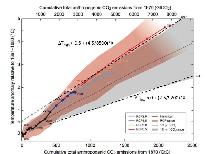
Commentary on the DECC Temperature rise calculations II • • The Calculator documentation makes it clear that in the web tool version, just the “Interactive CO 2 , CH 4, N 2 O, and SO 2 only” method is implemented, and option B is taken. The other method is only mentioned in the spreadsheet version of the Calculator , and (as the Spreadsheet User Guide explains on p 42 )“it is provided only as a reference calculation for the interested spreadsheet user within the spreadsheet”. The statistical analysis of the output data from ‘spaghetti diagrams’ (ie superimposed runs of many relatively independent computer climate models) has also made it possible to make statistical statements about the probabilities of various results, such as the Calculator statement in the Outputs-Emissions tab that “Cumulative emissions of 3010 Gt of CO 2 are associated with 50% of climate models achieving a 20 C temperature change” (the corresponding figure for 1. 5 o. C being given as 2260 Gt). These figures are also given in the web tool in the drop-down panel on emissions on the overview page) The Calculator team explicitly dissociates itself from taking the mid-point of the range of temperature figures quoted by the webtool as being a ‘best estimate’ (see the note in col AT line 84 of the Climate Impacts tab), and it also warns that the Calculator takes no account of the effect of other non-CO 2 gases (halocarbon, black carbon, VOCs, etc) or the climate-carbon feedback effect on the value of ΔT. There has recently been some research interest in the possible importance of hydrofluorocarbon gases in future years, because of their use as a replacement for banned CFCs and halons in refrigerators etc. It should be recorded that there is not universal agreement among climate scientists about the validity of the methodology for predicting climate changed used by the IPCC and the DECC Global Calculator team. Some scientific authors (eg Raymond Koch and Murry Salby) and some politicians (eg President-elect Donald Trump) seem to have radical doubts about the methodology.

Summary and Conclusions I • This paper explores the question in its sub-title: Did the 193 signatories of the UN Paris Agreement really know what they meant? The answer is ‘probably not’: they had no hard evidence that the target temperature rises agreed were achievable, given the physical, engineering and public opinion constraints on the energy system design. • This would matter less if the Paris Agreement had set firm ground-rules for an iterative global procedure to reach its targets. Sadly, it only established a system of national ‘declarations’, & a mechanism for further negotiations. What is required now is a much stronger scientific input to the discussions, based on good quantitative models. • The DECC Global Calculator is an (as yet unrivalled) software tool to support such discussions. It lets the user devise a model global energy system up to 2100, with numbers which are as accurate as are permitted by existing data (and credible future trends) on primary energy inputs and end-user outputs. • The Global Calculator has been through several iterations, but is still not fully fit for purpose. Changes are required to make it more user-friendly, and to improve its outputs on energy flows, emissions and temperature calculations. • One piece of good news is that since our earlier paper, we have found a procedure to generate a url from a 50 -line Excel pathway, allowing its transfer to the webtool. This greatly accelerates the process of ‘fine-tuning’ design pathways, and using webtool graphics

Summary and Conclusions II • Most uses of the Calculator to date have given rises significantly above 20 C, but until recently we had not managed to find better pathways. • Spurred on by this negative finding, in this paper, we have selected three of the Calculator’s ‘example’ pathways (WNA Allegro, CLIMACT and ICEPT) as starting points for an exploration to find credible ‘Paris-compliant’ pathways. These pathways represent three broadly different global energy strategies – ‘High Nuclear’, ‘High Renewable’ and ‘Intermediate’ (the last of which also includes a reasonably large amount of Carbon Capture & Storage). All three had ΔT < 2. 5 0 C. • Using information from the Calculator’s Output-Emissions tab, we inferred that the levers giving rise to the largest emission changes were nos 33 -48, so we explored the effect of variations in these levers (1 or 2 at a time) up to level 3. 0 or at most 3. 5. The result was that in every case ΔT could be decreased to ≤ 2. 1 0 C , and in some cases to ≤ 1. 6 0 C. Given the variance in the estimate of ΔT from a calculated cumulative emission in 2100, these could all be regarded as Paris-compliant. It is likely that with further ‘fine-tuning’, one could find pathways with still lower ΔT. • Variations with lever values of 3 - 3. 5 lie in the range characterised by DECC as ‘very’ or ‘extraordinarily’ ambitious , so we examined the Calculator’s assessment of their significance in each case. The level 3 variations seem to be reasonably achievable: the level 3. 5 variations would probably require much less welcome social & farming changes. More exploration is clearly required. Both British Pugwash and the EPS Energy Group would welcome collaborators!
- Slides: 26