GIS in the Sciences ERTH 4750 38031 Geostatistical

GIS in the Sciences ERTH 4750 (38031) Geo-statistical Computing and R Xiaogang (Marshall) Ma School of Science Rensselaer Polytechnic Institute Tuesday, February 12, 2013

We have learnt… • In lectures: – – – The concepts of GIS, geo-spatial data and information Geographic phenomena: fields, objects Computer representations: raster and vector Topology and spatial relationships Spatial referencing: vertical datum, horizontal datum Map projections • In labs: Map. Info Professional – File types, import external file formats, geocoding, creating points from coordinate information – Map objects, layers, selection and SQL selection, thematic map – Buffering, projection and printing

Written assignment 1 • Everyone received the email about written assignment 1? – http: //tw. rpi. edu/media/latest/GIS 2013_Assignment 1. pdf – Experimenting with projection, loading external data, querying, creating points from coordinate information, buffering, and printing functions in Map. Info Professional – 15% in final course grade – Submission method: written document by email to max 7@rpi. edu and Anastasia Rodzianko rodzia@rpi. edu – Due: Friday February 22, 2013 (by 5 pm EST) – Use office hours or email if meet challenges

Acknowledgements • The lecture of today is partly based on: – Rossiter, D. G. , 2012. Geo-statistical computing. Lecture in distance course Applied Geostatistics. ITC, University of Twente 4

Topics for this lecture 1. 2. 3. 4. 5. What is geostatistics The added value of geostatistics Feature and geographic spaces Geostatistical computing The R project for statistical computing 5

1 What is "geostatistics"? • What is "statistics"? • What then is "geo"-statistics? 6

1. 1 What is "statistics"? • The term "statistics" has two common meanings, which we want to clearly separate: descriptive and inferential statistics. • But to understand the difference between descriptive and inferential statistics, we must first be clear on the difference between populations and samples. 7

Populations and samples • A population is a set of well-defined objects – We must be able to say, for every object, if it is in the population or not – We must be able, in principle, to find every individual of the population A geographic example of a population is all pixels in a multi-spectral satellite image • A sample is a subset of a population – We must be able to say, for every object in the population, if it is in the sample or not – Sampling is the process of selecting a sample from a population Continuing the example, a sample from this population could be a set of pixels from known ground truth points 8

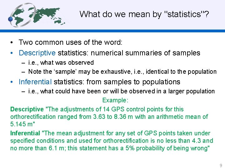
What do we mean by "statistics"? • Two common uses of the word: • Descriptive statistics: numerical summaries of samples – i. e. , what was observed – Note the ‘sample’ may be exhaustive, i. e. , identical to the population • Inferential statistics: from samples to populations – i. e. , what could have been or will be observed in a larger population Example: Descriptive "The adjustments of 14 GPS control points for this orthorectification ranged from 3. 63 to 8. 36 m with an arithmetic mean of 5. 145 m" Inferential "The mean adjustment for any set of GPS points taken under specified conditions and used for orthorectification is no less than 4. 3 and no more than 6. 1 m; this statement has a 5% probability of being wrong" 9

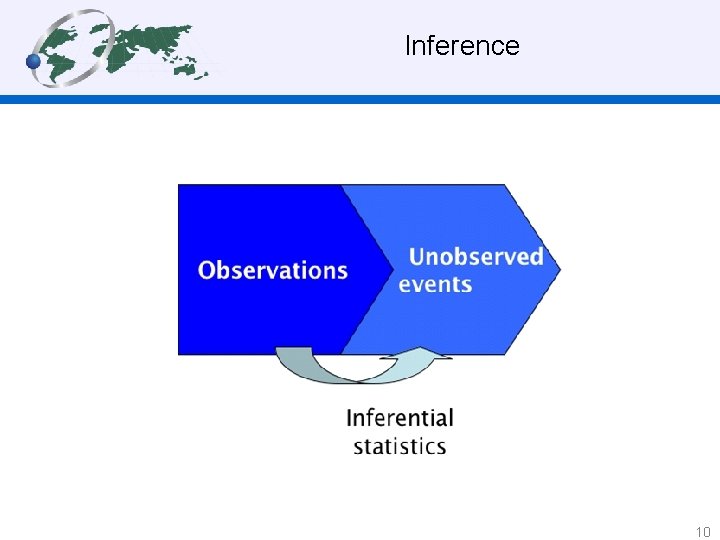
Inference 10

A concise definition of inferential statistics • Statistics: "The determination of the probable from the possible" – Davis, Statistics and Data Analysis in Geology, p. 6 • . . . which implies the rigorous definition and then quantification of "probable" – Probable causes of past events or observations – Probable occurrence of future events or observations • Then, a definition of inferential statistics: Observations ⇒ Inferences 11

• As humans, we infer constantly from the evidence around us. For example, I observe a person who can not walk a straight line, whose speech is slurred, and who smells strongly of alcohol - these are observable facts. I infer that the person is drunk - yet I didn’t see the person drink alcohol, and I haven’t analyzed the person’s blood alcohol level. Often we do not realize the line between observable facts and inferences • In statistical inference we quantify the degree of probability that our inference is true 12

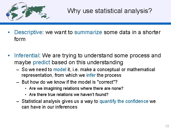
Why use statistical analysis? • Descriptive: we want to summarize some data in a shorter form • Inferential: We are trying to understand some process and maybe predict based on this understanding – So we need to model it, i. e. make a conceptual or mathematical representation, from which we infer the process – But how do we know if the model is "correct"? • Are we imagining relations where there are none? • Are there true relations we haven’t found? – Statistical analysis gives us a way to quantify the confidence we can have in our inferences 13

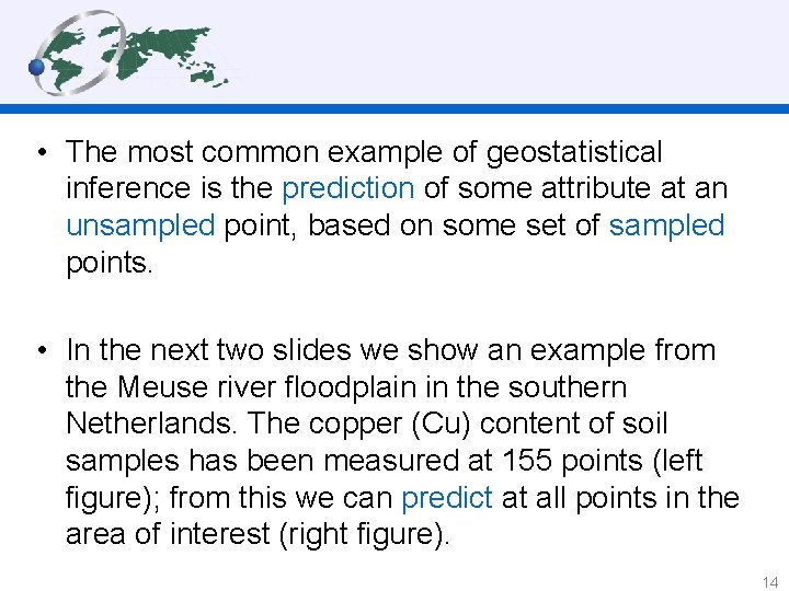
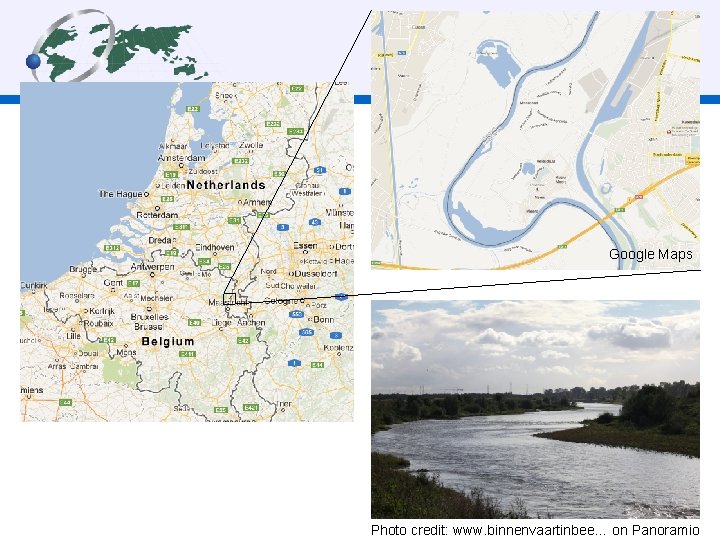
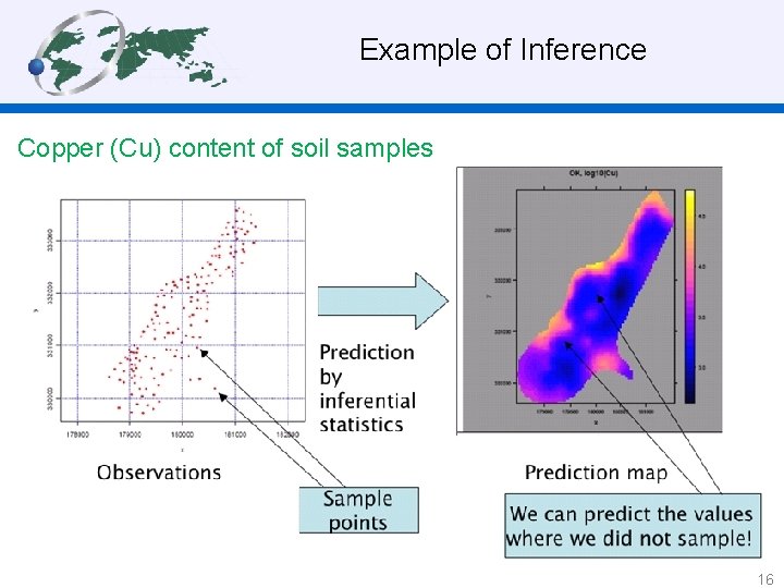
• The most common example of geostatistical inference is the prediction of some attribute at an unsampled point, based on some set of sampled points. • In the next two slides we show an example from the Meuse river floodplain in the southern Netherlands. The copper (Cu) content of soil samples has been measured at 155 points (left figure); from this we can predict at all points in the area of interest (right figure). 14

Google Maps Photo credit: www. binnenvaartinbee… on Panoramio

Example of Inference Copper (Cu) content of soil samples 16

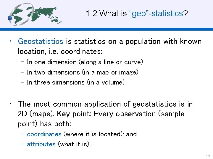
1. 2 What is “geo”-statistics? • Geostatistics is statistics on a population with known location, i. e. coordinates: – In one dimension (along a line or curve) – In two dimensions (in a map or image) – In three dimensions (in a volume) • The most common application of geostatistics is in 2 D (maps). Key point: Every observation (sample point) has both: – coordinates (where it is located); and – attributes (what it is). 17

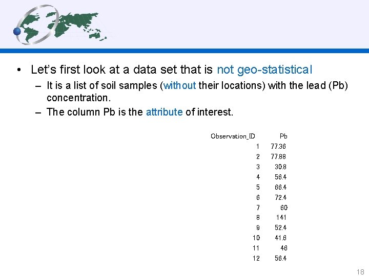
• Let’s first look at a data set that is not geo-statistical – It is a list of soil samples (without their locations) with the lead (Pb) concentration. – The column Pb is the attribute of interest. Observation_ID 1 2 3 4 5 6 7 8 9 10 11 12 Pb 77. 36 77. 88 30. 8 56. 4 66. 4 72. 4 60 141 52. 4 41. 6 46 56. 4 18

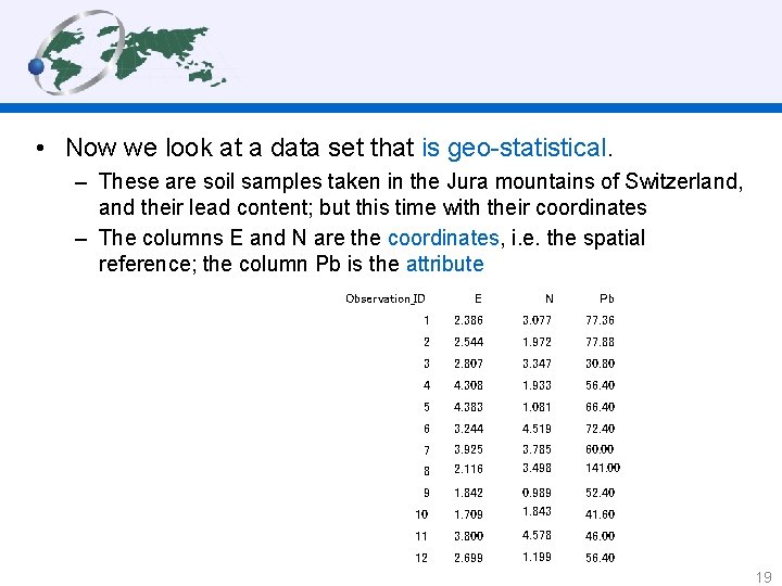
• Now we look at a data set that is geo-statistical. – These are soil samples taken in the Jura mountains of Switzerland, and their lead content; but this time with their coordinates – The columns E and N are the coordinates, i. e. the spatial reference; the column Pb is the attribute E N Pb 1 2. 386 3. 077 77. 36 2 2. 544 1. 972 77. 88 3 2. 807 3. 347 30. 80 4 4. 308 1. 933 56. 40 5 4. 383 1. 081 66. 40 6 3. 244 4. 519 72. 40 7 3. 925 8 2. 116 3. 785 3. 498 60. 00 141. 00 9 1. 842 52. 40 10 1. 709 0. 989 1. 843 11 3. 800 4. 578 46. 00 12 2. 699 1. 199 56. 40 Observation_ID 41. 60 19

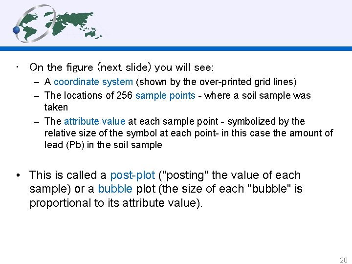
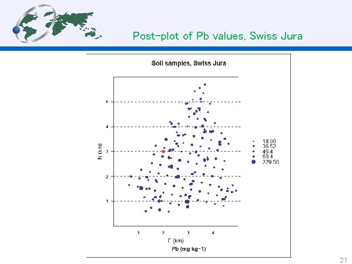
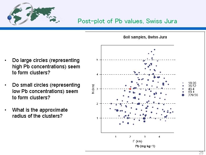
• On the figure (next slide) you will see: – A coordinate system (shown by the over-printed grid lines) – The locations of 256 sample points - where a soil sample was taken – The attribute value at each sample point - symbolized by the relative size of the symbol at each point- in this case the amount of lead (Pb) in the soil sample • This is called a post-plot ("posting" the value of each sample) or a bubble plot (the size of each "bubble" is proportional to its attribute value). 20

Post-plot of Pb values, Swiss Jura 21

• So, we know that each sample has a location. What is so special about that? After all, the attribute information is the same. What is the value-added of knowing the location? What new possibilities for analysis does this imply? 22

2 The added value of geostatistics • The location of a sample is an intrinsic part of its definition • All data sets from a given area are implicitly related by their coordinates – So they can be displayed and related in a GIS • Values at sample points can not be assumed to be independent: there is often evidence that nearby points tend to have similar values of attributes. – – • That is, there may be a spatial structure to the data Classical statistics assumes independence of samples But, if there is a spatial structure, this is not true! This has major implications for sampling design and statistical inference Data values may be related to their coordinates spatial trend 23

• Let’s look again at the post-plot, this time to see if we can discover evidence of spatial dependence that is, points that are close to each other have similar attribute values. 24

Post-plot of Pb values, Swiss Jura • Do large circles (representing high Pb concentrations) seem to form clusters? • Do small circles (representing low Pb concentrations) seem to form clusters? • What is the approximate radius of the clusters? 25

3 Feature and geographic spaces • The word space is used in mathematics to refer to any set of variables that form metric axes and which therefore allow us to compute a distance between points in that space. • If these variables represent geographic coordinates, we have a geographic space. • If these variables represent attributes, we have a feature space. 26

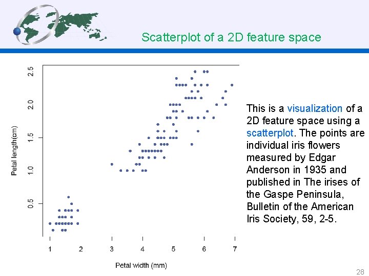
• It is important to understand these two uses of the word space, because we often want to contrast an analysis in feature space (not taking spatial position into account) with an analysis in geographic space (considering spatial position as the key element in the analysis). • Let's see an example of a feature space. This concept should be familiar from non-spatial statistics, although the term “feature space” may be new to you. 27

Scatterplot of a 2 D feature space This is a visualization of a 2 D feature space using a scatterplot. The points are individual iris flowers measured by Edgar Anderson in 1935 and published in The irises of the Gaspe Peninsula, Bulletin of the American Iris Society, 59, 2 -5. 28

3. 1 Feature space • This “space” is not geographic space, but rather a mathematical space formed by any set of variables: – Axes are the range of each variable – Coordinates are values of variables, possibly transformed or combined – The observations are related in this “space”, e. g. the “distance” between them can be calculated – We often plot variables in this space, e. g. scatterplots in 2 D or 3 D • Note: Feature space is sometimes referred to as attribute space. 29

• You are probably quite familiar with feature space from your study of non-spatial statistics. • Even with one variable, we have a unit of measure; this forms a 1 D or univariate feature space. • Most common are two variables which we want to relate with correlation or regression analysis; this is a bivariate feature space. • In multivariate analysis the feature space has more than two dimensions. 30

• Multivariate feature spaces can have many dimensions; we can only see three at a time. • The next slide is a visualization of a 3 D feature space using a 3 D-scatterplot. Again the observations are from the Anderson Iris data. 31

Scatterplot of a 3 D feature space Anderson Iris data 32

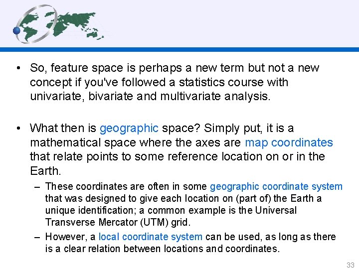
• So, feature space is perhaps a new term but not a new concept if you've followed a statistics course with univariate, bivariate and multivariate analysis. • What then is geographic space? Simply put, it is a mathematical space where the axes are map coordinates that relate points to some reference location on or in the Earth. – These coordinates are often in some geographic coordinate system that was designed to give each location on (part of) the Earth a unique identification; a common example is the Universal Transverse Mercator (UTM) grid. – However, a local coordinate system can be used, as long as there is a clear relation between locations and coordinates. 33

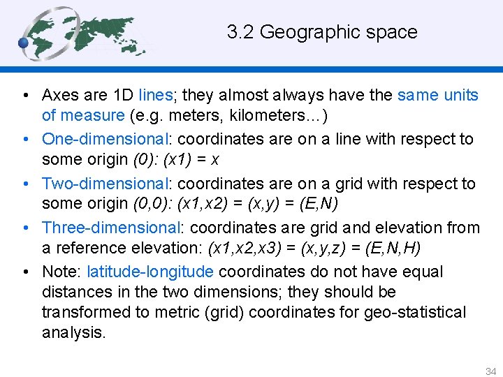
3. 2 Geographic space • Axes are 1 D lines; they almost always have the same units of measure (e. g. meters, kilometers…) • One-dimensional: coordinates are on a line with respect to some origin (0): (x 1) = x • Two-dimensional: coordinates are on a grid with respect to some origin (0, 0): (x 1, x 2) = (x, y) = (E, N) • Three-dimensional: coordinates are grid and elevation from a reference elevation: (x 1, x 2, x 3) = (x, y, z) = (E, N, H) • Note: latitude-longitude coordinates do not have equal distances in the two dimensions; they should be transformed to metric (grid) coordinates for geo-statistical analysis. 34

4 Geostatistical computing • Why geostatistical computing? • Geostatistical computing programs 35

4. 1 Why geostatistical computing? • Visualization: look for patterns in geographic and feature space; these suggest possible analyses – Is there a trend in the attributes with geographic position? e. g. rainfall decreasing away from an ocean – Is there local spatial dependence, i. e. values of points or polygons close by are more similar than those further apart? – Is there a spatial pattern to the sample points? • Computation: large numerical systems (e. g. the kriging system) that are practically impossible to solve by hand if there are more than a few points. 36

• It is impossible to consider geostatistical analysis without modern computing facilities. Here we list the many possibilities for geostatistical computing, along with a list of resources. • In this course we will use the R software environment for statistical computing and graphics, but we want to list the many alternatives and reasons you might choose one of them. 37

• There is a bewildering variety of software that deals with geostatistics. Some are commercial, some free. Some are part of a larger system (e. g. a GIS or a statistical computing environment), some stand-alone. Some only run on one operating system, some on many. Some are more comprehensive (more functionality) than others. What follows is only a partial list. • If you are connected to the internet, you can check the web links in the following pages for a few geostatistical software programs. 38

4. 2 What programs are available? • Lists – AI-GEOSTATS: A Web Resource for Geostatistic and Spatial Statistics – http: //www. ai-geostats. org/ – Freeware used for spatial statistics and geostatistics are listed under the “Software” button. • As a module of commercial GIS – Arc. GIS Geostatistical Analyst: http: //www. esri. com/software/arcgis/extensions/geostatistical/index. html • An extension to the commercial Arc. GIS program. A wide variety of procedures but weak documentation. – IDRISI: http: //www. clarklabs. org/products/ • From Clark Labs (US); a medium-cost GIS with good geostatistical functions. – ILWIS: http: //www. itc. nl/ilwis/ • From ITC (NL); almost free; with some geostatistical functions and excellent documentation (User's Guide Ch. 11, detailed on-line help). 39

• Stand-alone programs (1) – gstat: http: //www. gstat. org/ • Developed by Edzer Pebesma at Utrecht University (NL); we will use this as our primary tool but in the form of an R library. – gslib: http: //www. gslib. com/ • This is sophisticated code used by many advanced practioners. – Geo. EAS: http: //www. epa. gov/ada/csmos/models/geoeas. html • This was developed by the US Environmental Protection Agency and used for many regulatory studies. – SURFER: http: //www. goldensoftware. com/products/surfer. shtml • This commerical program has a wide variety of methods for making smooth surfaces or contour maps from point data. 40

• Stand-alone programs (2) – VESPER: http: //www. usyd. edu. au/su/agric/acpa/vesper. html • From the University of Syndey (AU), especially useful for interactive variogram modelling – FRAGSTATS: http: //www. umass. edu/landeco/research/fragstats. html • Landscape analysis 41

• Spreadsheets – These are designed for data manipulation; but they can also do matrix computations. Simple statistics are built-in as functions; and it is possible to program some geostatistical analysis with the matrix operations. – MS Excel (commerical): http: //www. microsoft. com/excel/ – Open. Office (open-source, free): http: //www. openoffice. org/ 42

• As part of a statistical computing environment (1) – R: http: //www. r-project. org/ – Open-source environment for statistical computing and visualization; includes several relevant packages, including (among others): • gstat: variogram modeling; simple, ordinary and universal point or block (co)kriging, sequential Gaussian or indicator (co)simulation • spatial: Functions for kriging and point pattern analysis • geo. R: Geostatistical analysis including traditional, likelihood-based and Bayesian methods • spdep: Spatial dependence: weighting schemes, statistics and models • spatstat: point pattern analysis • sp: underlying spatial data structures • DCluster: functions for the detection of spatial clusters of diseases 43

• As part of a statistical computing environment (1) – S-PLUS: http: //www. insightful. com/products/splus/default. asp – A commerical implementation of the S language with a comprehensive GUI. Has many of the same libraries as R. – Gen. Stat: http: //www. vsn-intl. co. uk/products/genstat/ – now commerical but originally conceived and developed at the Rothamsted Experimental Station (UK) 44

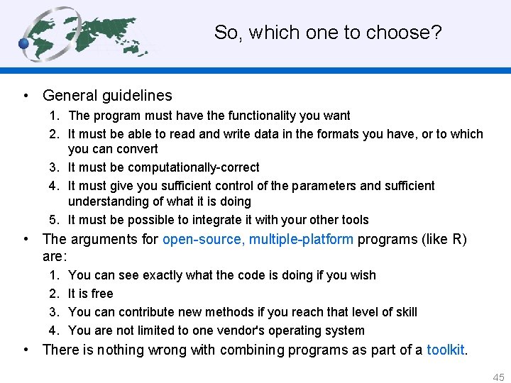
So, which one to choose? • General guidelines 1. The program must have the functionality you want 2. It must be able to read and write data in the formats you have, or to which you can convert 3. It must be computationally-correct 4. It must give you sufficient control of the parameters and sufficient understanding of what it is doing 5. It must be possible to integrate it with your other tools • The arguments for open-source, multiple-platform programs (like R) are: 1. 2. 3. 4. You can see exactly what the code is doing if you wish It is free You can contribute new methods if you reach that level of skill You are not limited to one vendor's operating system • There is nothing wrong with combining programs as part of a toolkit. 45

5 The R project for statistical computing • What is it? • Why do we use it? 46

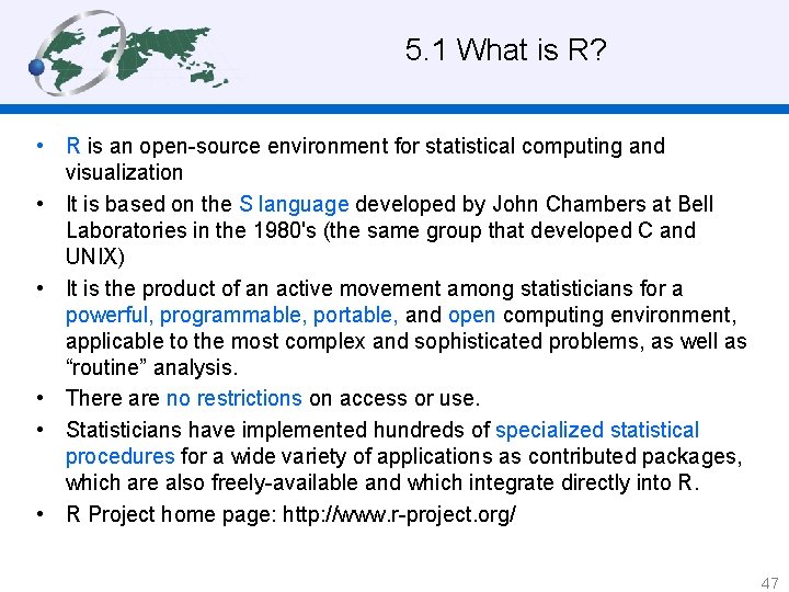
5. 1 What is R? • R is an open-source environment for statistical computing and visualization • It is based on the S language developed by John Chambers at Bell Laboratories in the 1980's (the same group that developed C and UNIX) • It is the product of an active movement among statisticians for a powerful, programmable, portable, and open computing environment, applicable to the most complex and sophisticated problems, as well as “routine” analysis. • There are no restrictions on access or use. • Statisticians have implemented hundreds of specialized statistical procedures for a wide variety of applications as contributed packages, which are also freely-available and which integrate directly into R. • R Project home page: http: //www. r-project. org/ 47

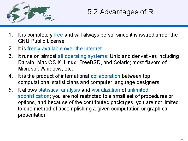
5. 2 Advantages of R 1. It is completely free and will always be so, since it is issued under the GNU Public License 2. It is freely-available over the internet 3. It runs on almost all operating systems: Unix and derivatives including Darwin, Mac OS X, Linux, Free. BSD, and Solaris; most flavors of Microsoft Windows, etc. 4. It is the product of international collaboration between top computational statisticians and computer language designers 5. It allows statistical analysis and visualization of unlimited sophistication; you are not restricted to a small set of procedures or options, and because of the contributed packages, you are not limited to one method of accomplishing a given computation or graphical presentation 48

Advantages of R (2) 6. It can work on objects of unlimited size and complexity 7. It can exchange data in MS-Excel, text, fixed and delineated formats (e. g. CSV), so that existing datasets are easily imported, and results computed in R are easily exported 8. It is supported by comprehensive technical documentation and usercontributed tutorials. There also several good textbooks on statistical methods that use R for illustration 9. Every computational step is recorded, and this history can be saved for later use or documentation 10. It stimulates critical thinking about problem-solving rather than a “push the button” mentality 49

Advantages of R (3) 11. It is fully programmable, with its own sophisticated computer language, named S; 12. Repetitive procedures can easily be automated by user-written scripts or functions; 13. All source code is published, so you can see the exact algorithms being used; also, expert statisticians can make sure the code is correct. 50

5. 3 Disadvantages of R 1. The default Windows and Mac OS X graphical user interface (GUI) is limited to simple system interaction and does not include statistical procedures. The user must type commands to enter data, do analyses, and plot graphs. But. . . this has the advantage that you have complete control over the system. Note: The Rcmdr add-on package provides a reasonable GUI for common tasks. 2. The user must decide on the sequence of analyses and execute them step-by-step. However, it is easy to create scripts with all the steps in an analysis, and run the script from the command line or menus. But. . . this has the advantage that you can save the processing log of all your analysis steps and their results for inclusion in reports or re-use. 51

Disadvantages of R (2) 3. The user must learn a new way of thinking about data, as objects each with its class, which in turn supports a set of methods. But. . . this has the advantage that you can only operate on an object according to methods that make sense for it. 4. The user must learn the S language, both for commands and the notation used to specify statistical models. However, this allows the user to specify models using a compact and consistent notation. 52

• For the purposes of this course/module we only need to learn a limited part of what R can offer; perhaps after the course you will be motivated to learn more. • R is a very complex program with unlimited possibilities. The best way to learn it is step-by-step, from the basics to the more complex. In this first lecture we will not do any geo-statistics; the computer exercise will illustrate the basic operation of R. 53

6 Learning resources • Geostatistics textbooks • Useful web pages • Resources for learning R This section is included for your reference 54

Geostatistics texts: Mathematical • Diggle, P. J. and Ribeiro Jr, P. J. , 2007. Model-based geostatistics. Springer. • Chiles, J. -P. and Delner, P. , 1999. Geostatistics: modeling spatial uncertainty. Wiley series in probability and statistics. John Wiley & Sons, New York. • Christakos, G. , 2000. Modern spatiotemporal geostatistics. Oxford University Press, New York. • Cressie, N. , 1993. Statistics for spatial data. John Wiley & Sons, New York. • Ripley, B. D. , 1981. Spatial statistics. John Wiley & Sons, New York. 55

Geostatistics texts: Particular application field • Davis, J. C. , 2002. Statistics and data analysis in geology. John Wiley & Sons, New York. • Fotheringham, A. S. , Brunsdon, C. and Charlton, M. , 2000. Quantitative geography: perspectives on spatial data analysis. Sage Publications, London ; Thousand Oaks, Calif. • Stein, A. , Meer, F. v. d. and Gorte, B. G. F. (Editors), 1999. Spatial statistics for remote sensing. Kluwer Academic, Dordrecht. • Kitanidis, P. K. , 1997. Introduction to geostatistics : applications to hydrogeology. Cambridge University Press, Cambridge, England. 56

Geostatistics texts: Application-oriented but mathematical • Webster, R. , and Oliver, M. A. , 2001. Geostatistics for environmental scientists. Wiley & Sons, Chichester. • Goovaerts, P. , 1997. Geostatistics for natural resources evaluation. Oxford University Press, Oxford and New York. • Isaaks, E. H. and Srivastava, R. M. , 1990. An introduction to applied geostatistics. Oxford University Press, New York. 57

Geostatistics texts: Emphasis on computational methods • Venables, W. N. & Ripley, B. D. , 2002. Modern applied statistics with S, 4 th edition. Springer-Verlag, New York. For the serious R user. This covers a wide variety of modern statistical methods, including spatial statistics. • Deutsch, C. V. , & Journel, A. G. , 1992. GSLIB: Geostatistical software library and user's guide. Oxford University Press, Oxford. 58

Web pages • Statistics – Electronic Statistics Textbook from Stat. Soft: http: //www. statsoft. com/textbook/stathome. html – NIST/SEMATECH e-Handbook of Statistical Methods: http: //www. itl. nist. gov/div 898/handbook/ • Geostatistics – R task view: Analysis of Spatial Data http: //cran. r-project. org/web/views/Spatial. html – Geostatistical analysis tutor, mainly aimed at mining applications: http: //www. uncert. com/tutor/ 59

Resources for learning R • These are not necessary for this course; they are listed for your reference in case you decide to continue with R. • General introductions – Venables, W. N. ; Smith, D. M. ; R Development Core Team, 2006. An Introduction to R (Notes on R: A Programming Environment for Data Analysis and Graphics), Version 2. 4. 0 (2006 -10 -03). http: //www. cran. r-project. org – Rossiter, D. G. , 2006. Introduction to the R Project for Statistical Computing for use at ITC, Enschede (NL), 116 pp. http: //www. itc. nl/personal/rossiter/teach/R/RIntro_ITC. pdf 60

• Textbooks using R – Dalgaard, P. 2002. Introductory Statistics with R. Springer Verlag. This is a clearly-written introduction to statistics, using R in all examples. – Venables, W. N. & Ripley, B. D. 2002. Modern applied statistics with S. New York: Springer-Verlag, 4 th edition; http: //www. stats. ox. ac. uk/pub/MASS 4/ Presents a wide variety of up-to-date statistical methods (including spatial statistics) with algorithms coded in S; includes an introduction to R, R programming, and R graphics. – Fox, J. 2002. An R and S-PLUS Companion to Applied Regression. Newbury Park: Sage. A social scientists explains how to use R for regression analysis, including advanced techniques; this is a companion to his text: Fox, J. 1997. Applied regression, linear models, and related methods. Newbury Park: Sage 61

• Technical Notes using R – D G Rossiter has written a number of technical notes showing how to accomplish some statistical tasks with R; the full list is at: http: //www. itc. nl/personal/rossiter/pubs/list. html#pubs_m_R These include general data analysis, logistic regression, confusion matrices, co-kriging, partioning transects, and tting rational functions 62

Assignment for this week • Reading: Install the R computing environment • Preparation: Install R environment before Fri. lab • Written Assignment 1 63

Next classes • Friday class: – R environment: • • Loading & examining example dataset Descriptive statistics Exploratory graphics Linear modeling • In preparation: – Next Tuesday: Exploring and visualizing spatial data 64