Geospatial Modeling Maps and Animated Geography E Lynn

Geospatial Modeling Maps and Animated Geography E. Lynn Usery Professor, University of Georgia Research Geographer, U. S. Geological Survey

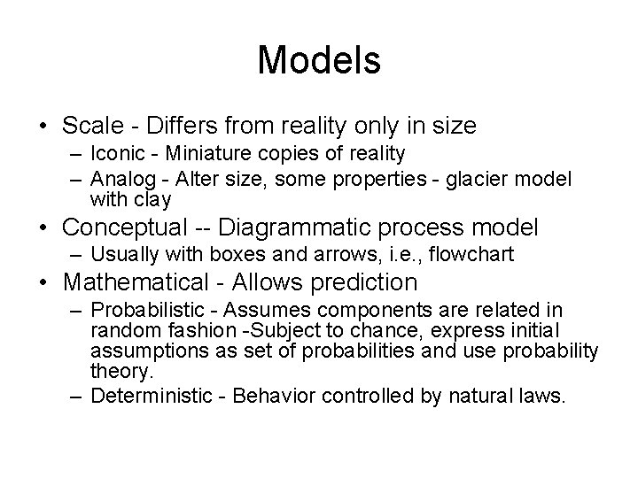
Models • Scale - Differs from reality only in size – Iconic - Miniature copies of reality – Analog - Alter size, some properties - glacier model with clay • Conceptual -- Diagrammatic process model – Usually with boxes and arrows, i. e. , flowchart • Mathematical - Allows prediction – Probabilistic - Assumes components are related in random fashion -Subject to chance, express initial assumptions as set of probabilities and use probability theory. – Deterministic - Behavior controlled by natural laws.

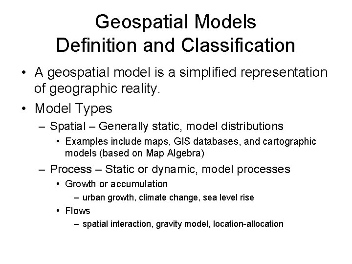
Geospatial Models Definition and Classification • A geospatial model is a simplified representation of geographic reality. • Model Types – Spatial – Generally static, model distributions • Examples include maps, GIS databases, and cartographic models (based on Map Algebra) – Process – Static or dynamic, model processes • Growth or accumulation – urban growth, climate change, sea level rise • Flows – spatial interaction, gravity model, location-allocation

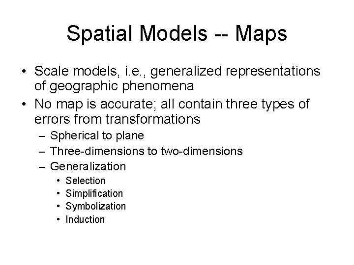
Spatial Models -- Maps • Scale models, i. e. , generalized representations of geographic phenomena • No map is accurate; all contain three types of errors from transformations – Spherical to plane – Three-dimensions to two-dimensions – Generalization • • Selection Simplification Symbolization Induction

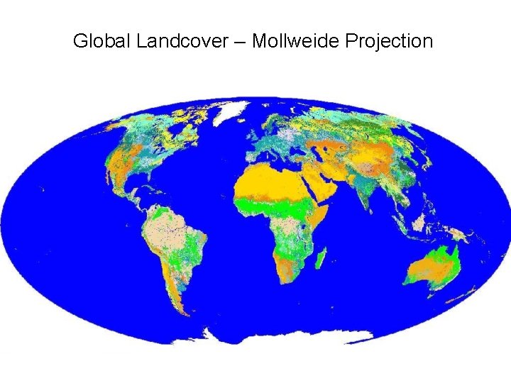
Global Landcover – Mollweide Projection

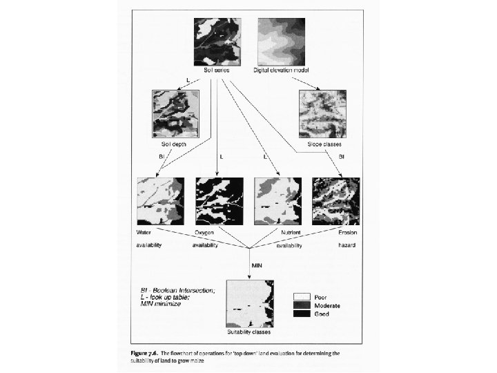
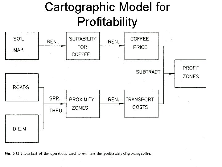
Spatial Models--Cartographic Models • Map themes again geographically registered but combined with a sequence of operations (map algebra) that generate a desired result from a set of basic input data layers • Map layers become variables in map algebra with operators on and between variables • Operators include point, neighborhood, and global • Most commonly implemented with raster data layers

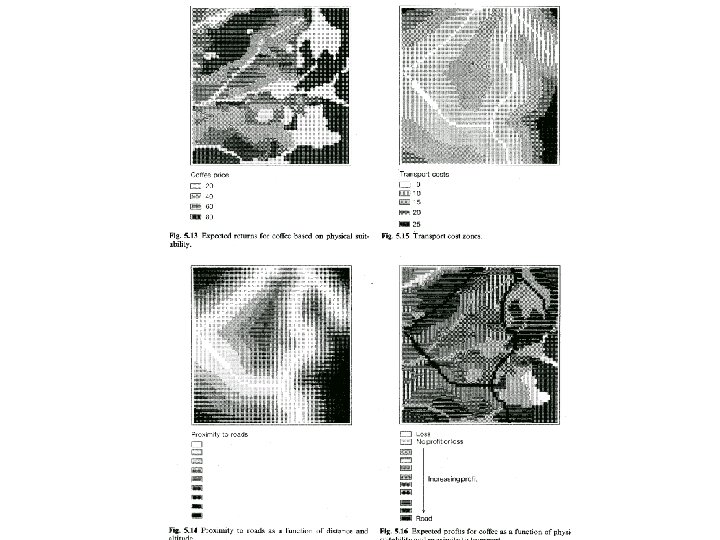
Cartographic Model for Profitability

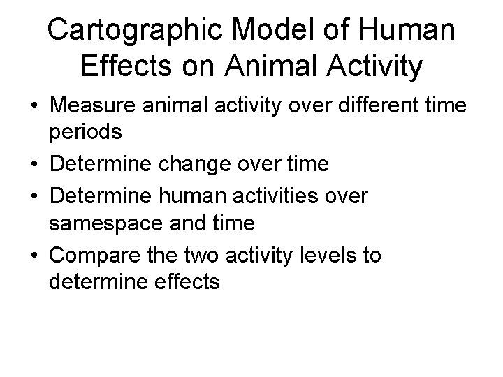
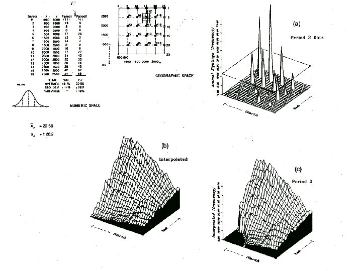
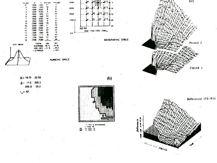
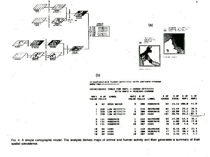
Cartographic Model of Human Effects on Animal Activity • Measure animal activity over different time periods • Determine change over time • Determine human activities over samespace and time • Compare the two activity levels to determine effects

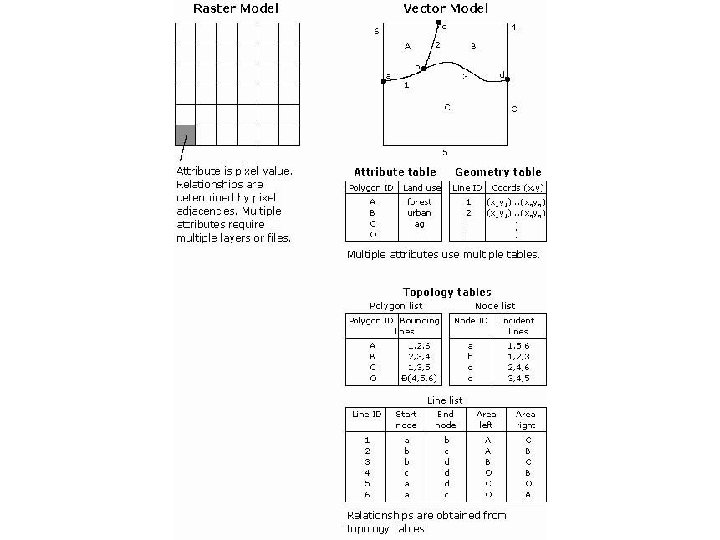
Spatial Models-- GIS Databases • Map model placed in computer representation • Includes all error inherent in the map model • Usually include multiple maps of individual themes registered to a common spheroid, datum, projection, and coordinate system with associated attributes linked to geographic object (point, line, area) identifiers commonly stored in a relational database

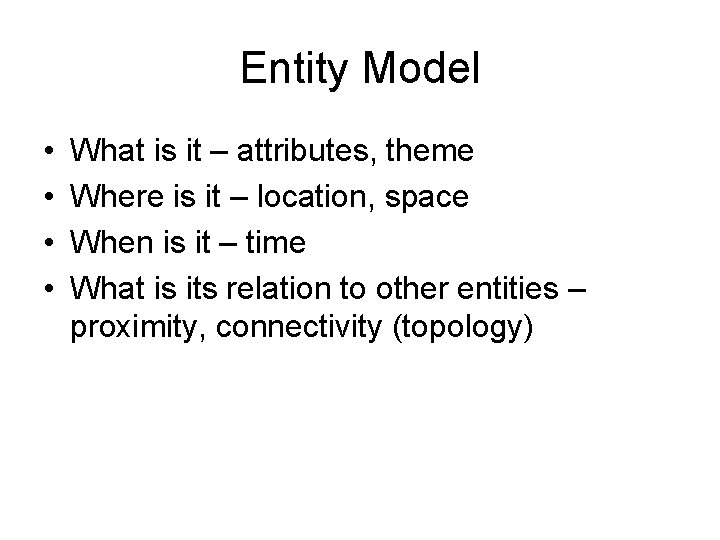
Entity Model • • What is it – attributes, theme Where is it – location, space When is it – time What is its relation to other entities – proximity, connectivity (topology)

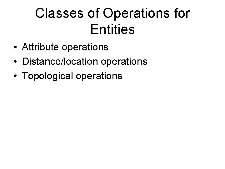
Classes of Operations for Entities • Attribute operations • Distance/location operations • Topological operations

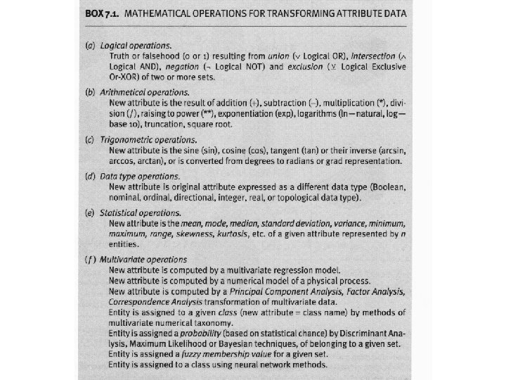
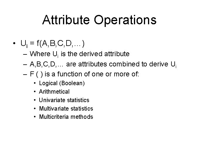
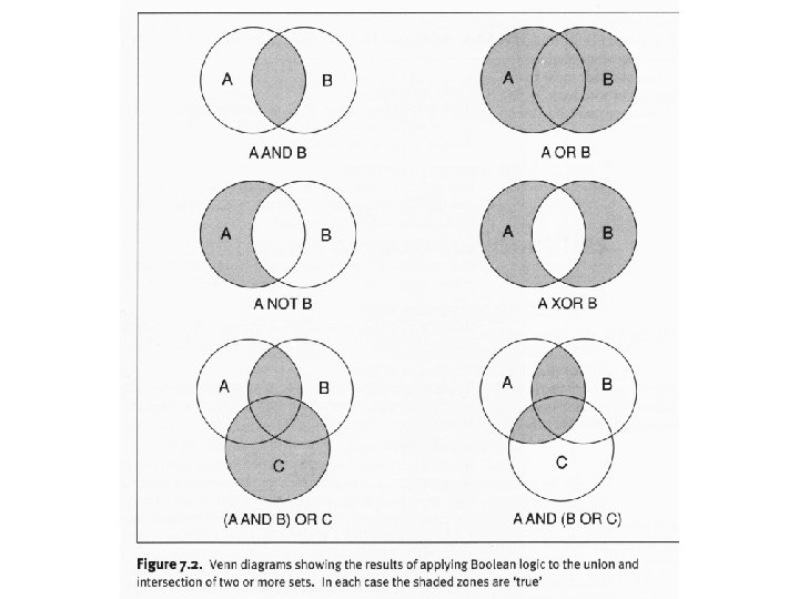
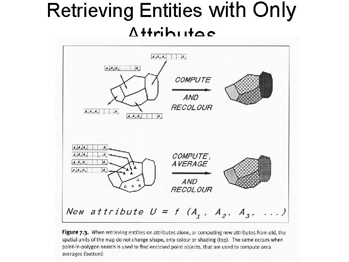
Attribute Operations • Ui = f(A, B, C, D, …) – Where Ui is the derived attribute – A, B, C, D, … are attributes combined to derive Ui – F ( ) is a function of one or more of: • • • Logical (Boolean) Arithmetical Univariate statistics Multicriteria methods

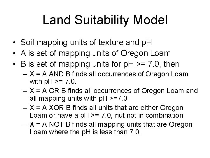
Land Suitability Model • Soil mapping units of texture and p. H • A is set of mapping units of Oregon Loam • B is set of mapping units for p. H >= 7. 0, then – X = A AND B finds all occurrences of Oregon Loam with p. H >= 7. 0. – X = A OR B finds all occurrences of Oregon Loam and all mapping units with p. H >=7. 0. – X = A XOR B finds all units that are either Oregon Loam or have a p. H >= 7. 0, nut not in combination – X = A NOT B finds all mapping units that are Oregon Loam where the p. H is less than 7. 0.

Retrieving Entities with Only Attributes

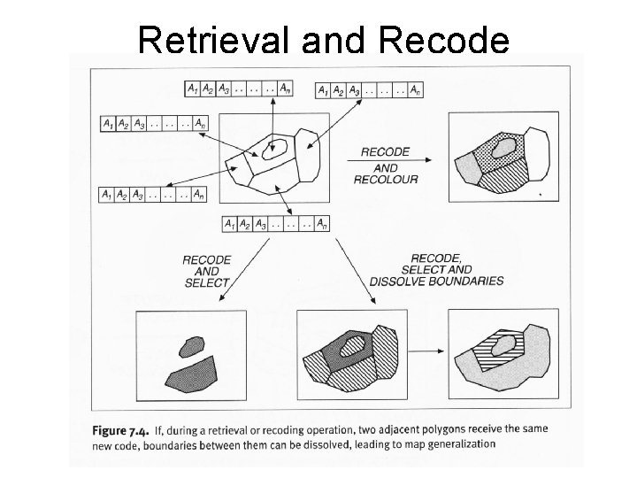
Retrieval and Recode

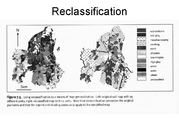
Reclassification

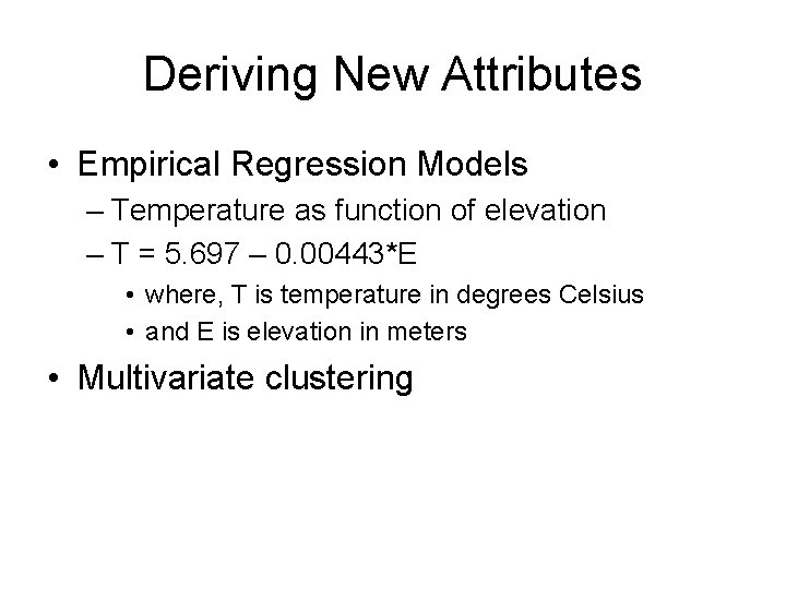
Deriving New Attributes • Empirical Regression Models – Temperature as function of elevation – T = 5. 697 – 0. 00443*E • where, T is temperature in degrees Celsius • and E is elevation in meters • Multivariate clustering

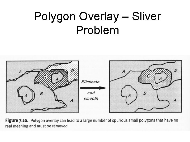
Polygon Overlay – Sliver Problem

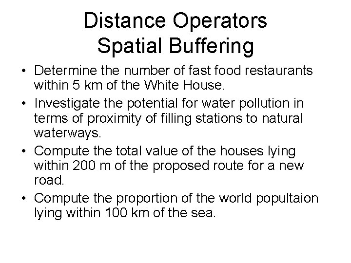
Distance Operators Spatial Buffering • Determine the number of fast food restaurants within 5 km of the White House. • Investigate the potential for water pollution in terms of proximity of filling stations to natural waterways. • Compute the total value of the houses lying within 200 m of the proposed route for a new road. • Compute the proportion of the world popultaion lying within 100 km of the sea.

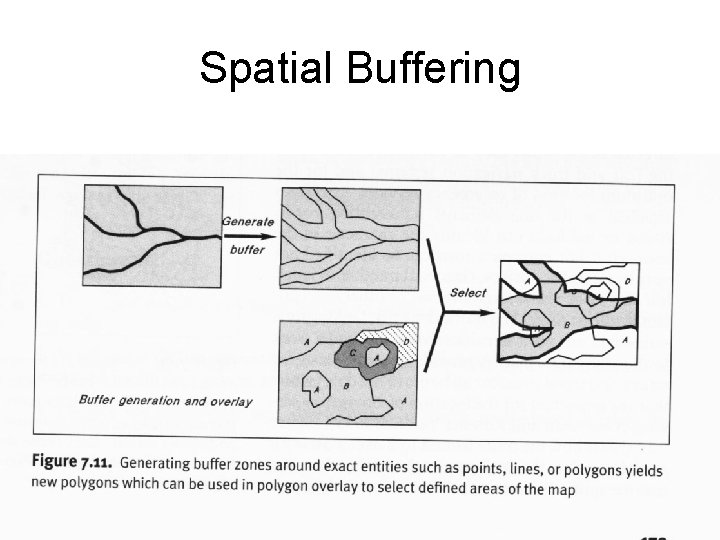
Spatial Buffering

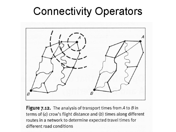
Connectivity Operators

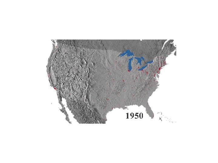
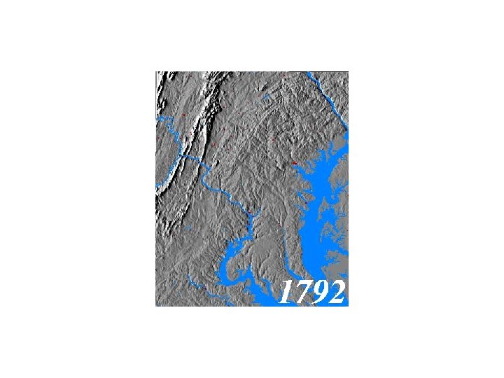
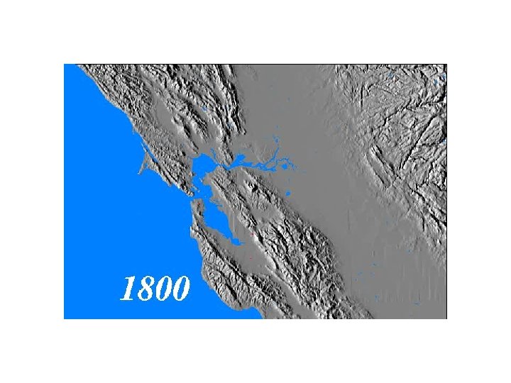
Geospatial Process Models • Often use results of GIS Databases as steps in a process • Non-point Source Pollution -- AGNPS • Sea Level Rise • Urban Growth -- SLEUTH

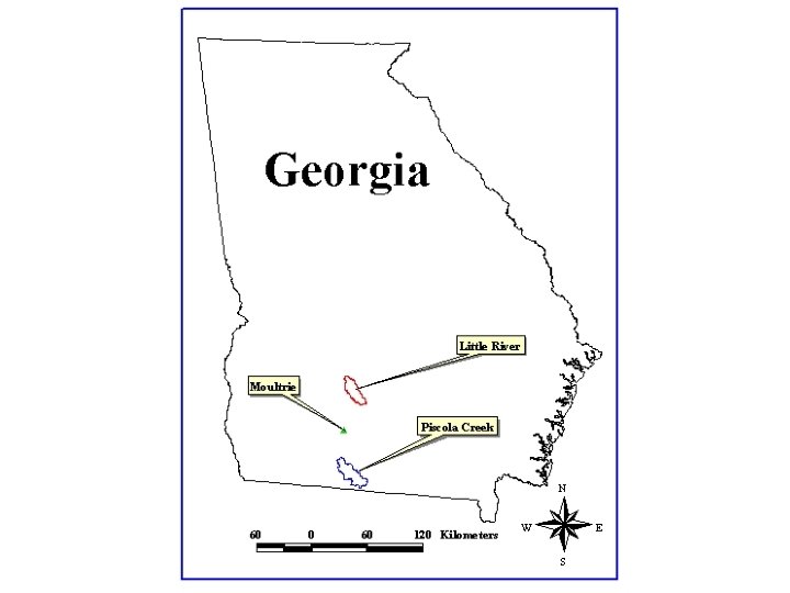
AGNPS • Agricultural Non-Point Pollution Source

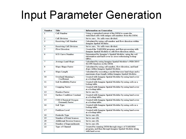
Introduction -- AGNPS • Operates on a cell basis and is a distributed parameter, event-based model • Requires 22 input parameters • Elevation, land cover, and soils data are the base for extraction of input parameters

Input Parameter Generation • 22 parameters; varying degrees of computational development – Simple, straightforward, complex

Input Parameter Generation

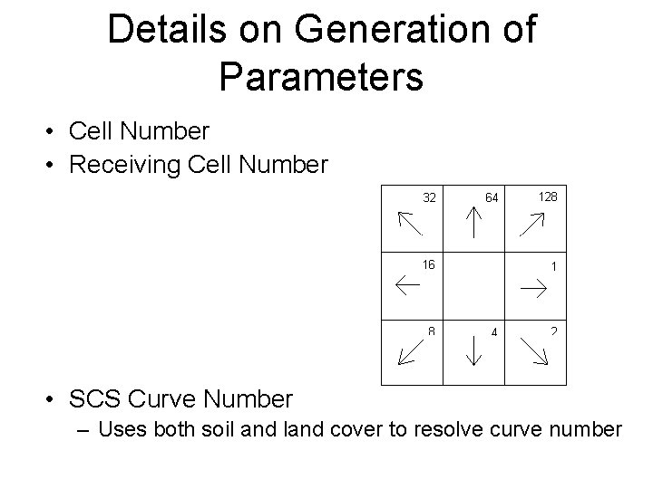
Details on Generation of Parameters • Cell Number • Receiving Cell Number • SCS Curve Number – Uses both soil and land cover to resolve curve number

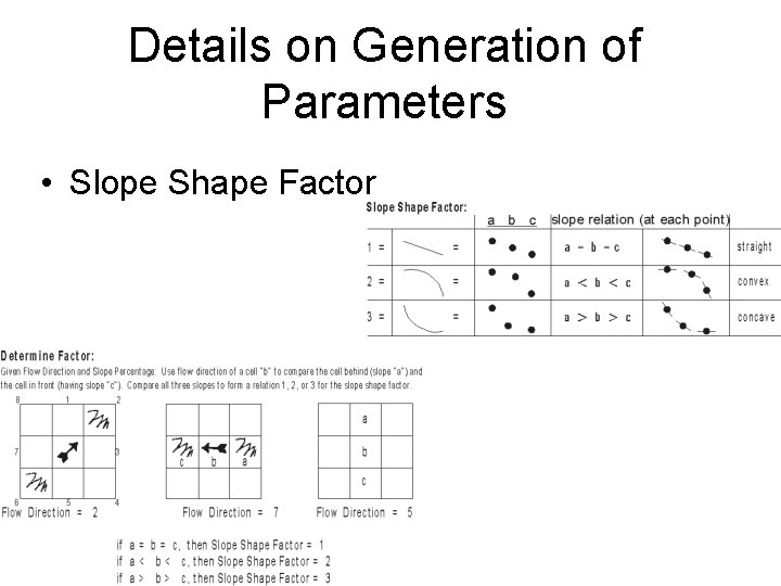
Details on Generation of Parameters • Slope Shape Factor

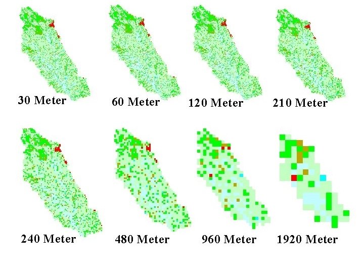
Extraction Methods • Used object-oriented programming and macro languages – C/ C++ and EML • Manipulated the raster GIS databases with Imagine • Extracted parameters for each resolution for both boundaries using AGNPS Data Generator

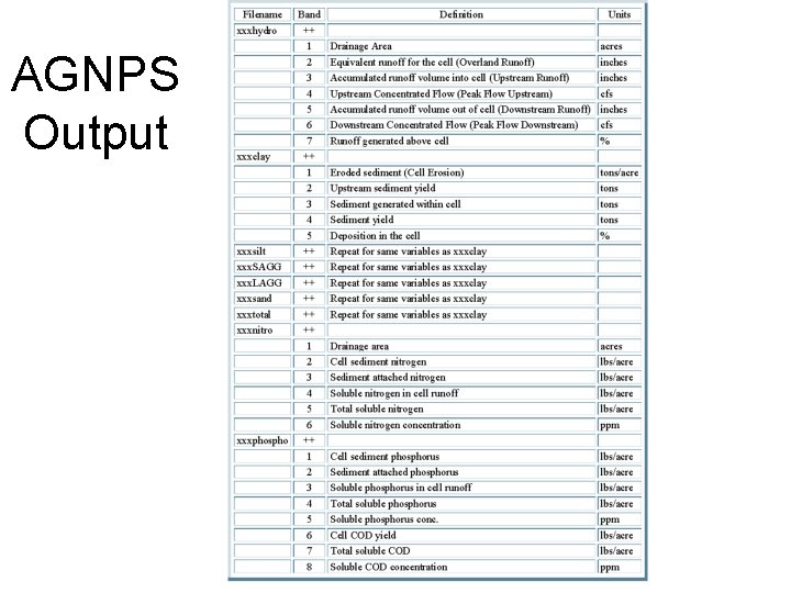
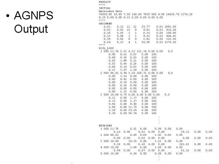
Creating AGNPS Output • AGNPS creates a nonpoint source (“. nps”) file • ASCII file like the input; tabular, numerical form

AGNPS Output

• AGNPS Output

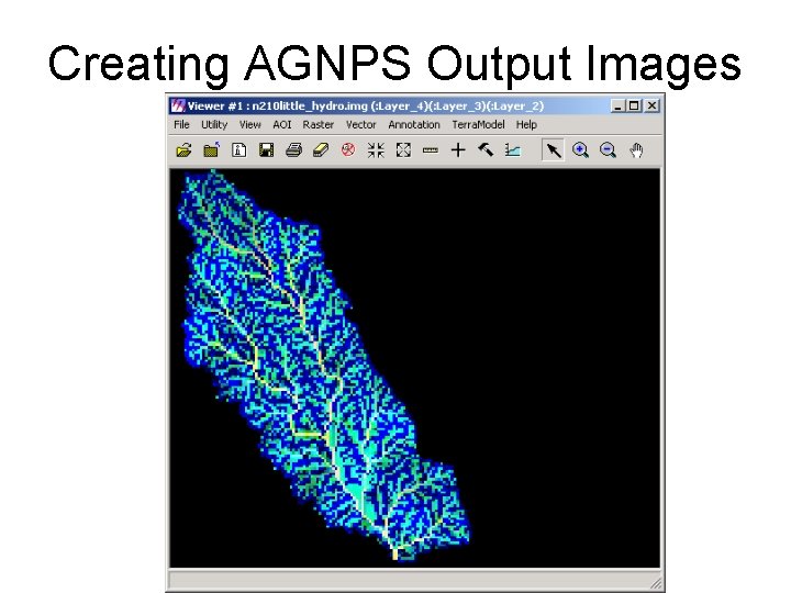
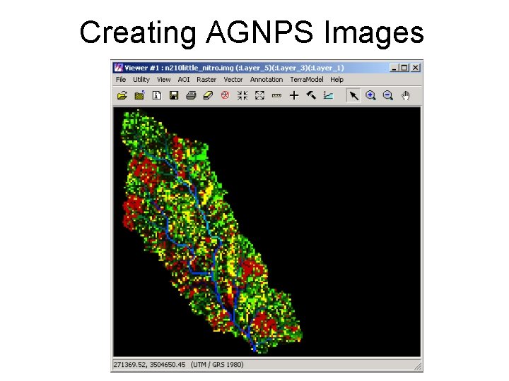
Creating AGNPS Output Images • Output Image Creation – Combined “. nps” file with Parameter 1 to create multidimensional images – Users can graphically display AGNPS output – Process: create image with “x” layers, fill layers with AGNPS output data, set projection and stats for image – Multi-layered (bands) images per model event

Creating AGNPS Output Images

Creating AGNPS Images

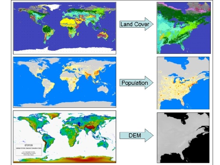
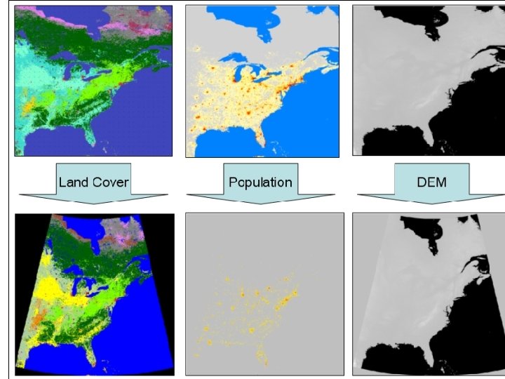
Model of Sea Level Rise • Data inputs – Elevation – Gtopo 30 – Population -- Landscan – Land Cover – Global Land Cover • 30 arc-sec resolution cells (approximately 1 km at the Equator) • Most accurate global data available • Model for eastern North America only

Urban Growth -- SLEUTH • Model of converting land to urban from other uses • Cellular Automata model based on probabilities from Monte Carlo stochastic simulation • Model begins with an existing urban base (i. e, some cells are urban and others nonurban based on historical land cover data)

Urban Growth -- SLEUTH • Non-urban cells change to urban based on 7 controlling variables (GIS layers) and user specified parameters controlling growth • Variables: Slope, Land Cover, Elevation, Urban, Transportation, Hillshade • Types of growth: – – Spontaneous Growth New Spreading Centers Edge Growth Road-Influenced Growth