Geospatial Analysis II proximity buffers cost surfaces Geospatial

Geospatial Analysis II: proximity, buffers, cost surfaces Geospatial Analysis and Modeling: Lecture notes Helena Mitasova, NCSU MEAS

Project Two page revised proposal due - see the schedule for date: • • Introduction: background, statement of the problem, motivation Objective or research question Site and data – coordinates, coordinate system, units – list of data sets: already in GIS, still need to download – images showing your location and sample of data that you have Approach: general methodology or workflow to accomplish the objective Expected results: what information will your analysis and modeling provide and in what form (maps, tables, graphs, etc). References: list of 5 -10 research papers that address similar topic that provide the motivation for your project, inspire the approach that you can improve upon, provide sources for your data. Web documents are OK but at least some should be research papers.

Outline • • measuring distance buffers cost surfaces least cost path

Measuring distance Distance: • Euclidean: shortest distance in plane • Geodesic: shortest distance over curved surface, great circle on sphere: orthodrome equation: http: //mathworld. wolfram. com/Great. Circle. html • Rhumbline (loxodrome): constant bearing path, line in Mercator projection, NOT the shortest path equation: http: //en. wikipedia. org/wiki/Rhumb_line

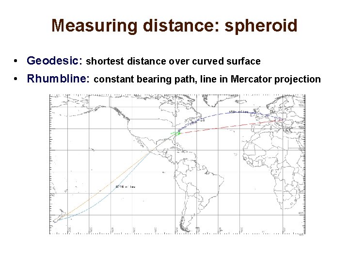
Measuring distance: spheroid • Geodesic: shortest distance over curved surface • Rhumbline: constant bearing path, line in Mercator projection

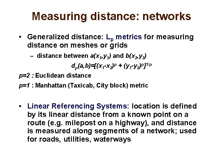
Measuring distance: networks • Generalized distance: Lp metrics for measuring distance on meshes or grids – distance between a(x 1, y 1) and b(x 2, y 2) dp(a, b)=[(x 1 -x 2)p + (y 1 -y 2)p]1/p p=2 : Euclidean distance p=1 : Manhattan (Taxicab, City block) metric • Linear Referencing Systems: location is defined by its linear distance from a known point on a route (e. g. milepost on a highway), and distance is measured along segments of a network; used for roads, utilities, waterways

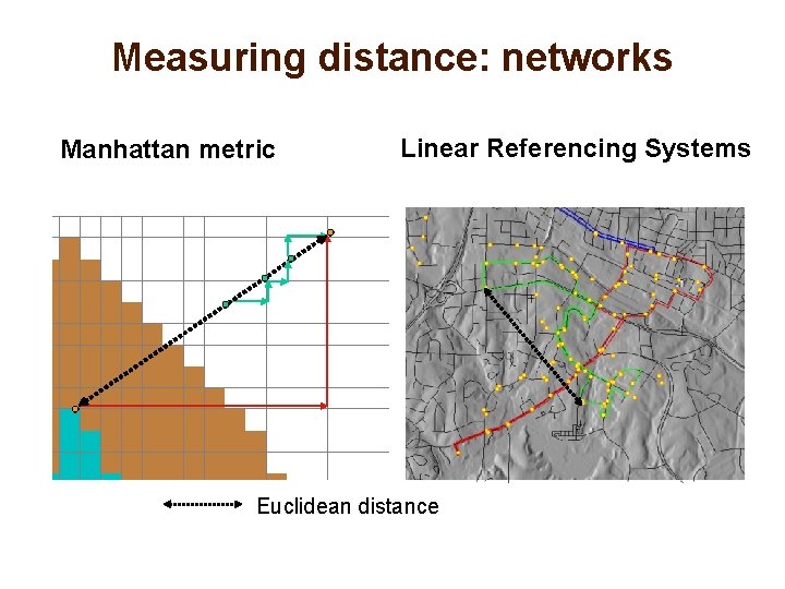
Measuring distance: networks Manhattan metric Linear Referencing Systems Euclidean distance

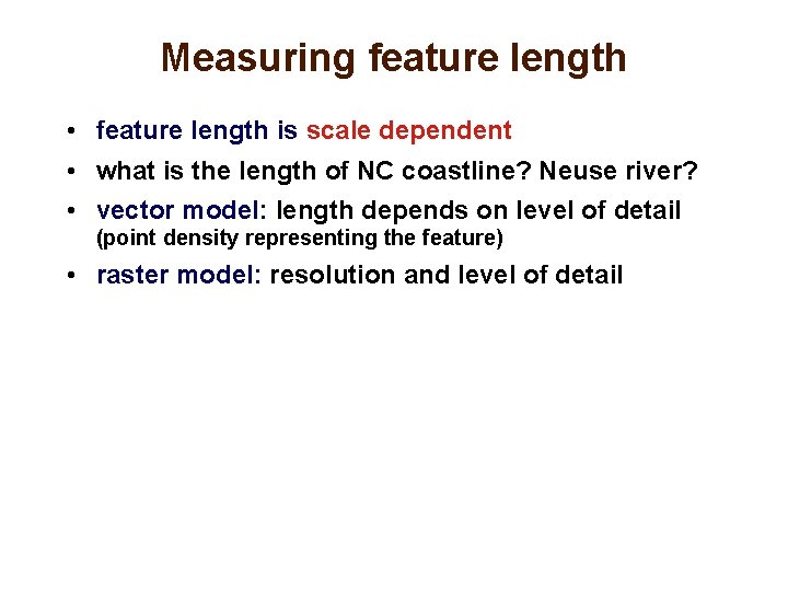
Measuring feature length • feature length is scale dependent • what is the length of NC coastline? Neuse river? • vector model: length depends on level of detail (point density representing the feature) • raster model: resolution and level of detail

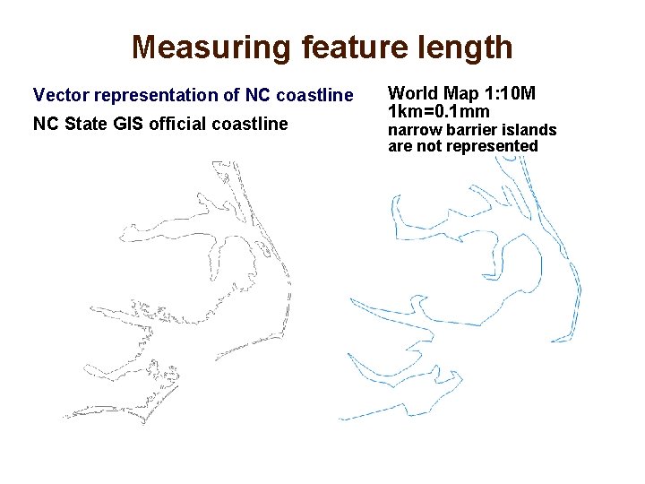
Measuring feature length Vector representation of NC coastline NC State GIS official coastline World Map 1: 10 M 1 km=0. 1 mm narrow barrier islands are not represented

Raster map buffer operations Proximity analysis function • creates buffer zones (equal distance zones) from a given feature (point, line or area) • applies to raster map layers representing discrete objects • resolution should be sufficiently higher (cell size should be n-times smaller) than distances (buffer widths)

Raster map buffer: lines Draws the requested distance rings around each cell with the given category: line buffer example

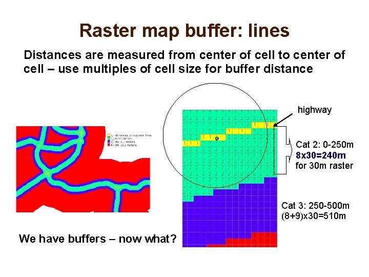
Raster map buffer: lines Distances are measured from center of cell to center of cell – use multiples of cell size for buffer distance highway Cat 2: 0 -250 m 8 x 30=240 m for 30 m raster Cat 3: 250 -500 m (8+9)x 30=510 m We have buffers – now what?

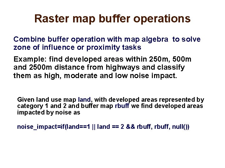
Raster map buffer operations Combine buffer operation with map algebra to solve zone of influence or proximity tasks Example: find developed areas within 250 m, 500 m and 2500 m distance from highways and classify them as high, moderate and low noise impact. Given land use map land, with developed areas represented by category 1 and 2 and buffer map rbuff we find developed areas impacted by noise as noise_impact=if(land==1 || land == 2 && rbuff, null())

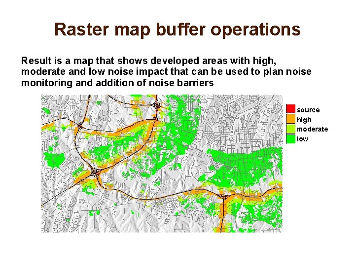
Raster map buffer operations Result is a map that shows developed areas with high, moderate and low noise impact that can be used to plan noise monitoring and addition of noise barriers source high moderate low

Raster map buffer operations Are there any schools affected in high and moderate noise area? If yes, how many students? How can we find how many people are affected ? Can we do an accurate estimate? Given the school capacity raster map school_cap and buffer map rbuff we find schools impacted by noise as schools_noise=if(school_cap && rbuff < 4, school_cap, null()) number of students affected r. sum schools_noise Note: To create schools_cap map we convert vector point map to raster using capacity attribute for value and school name for label

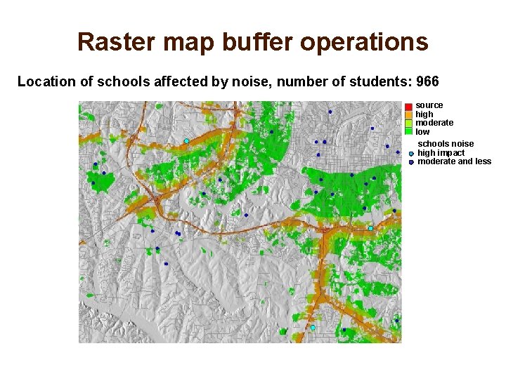
Raster map buffer operations Location of schools affected by noise, number of students: 966 source high moderate low schools noise high impact moderate and less

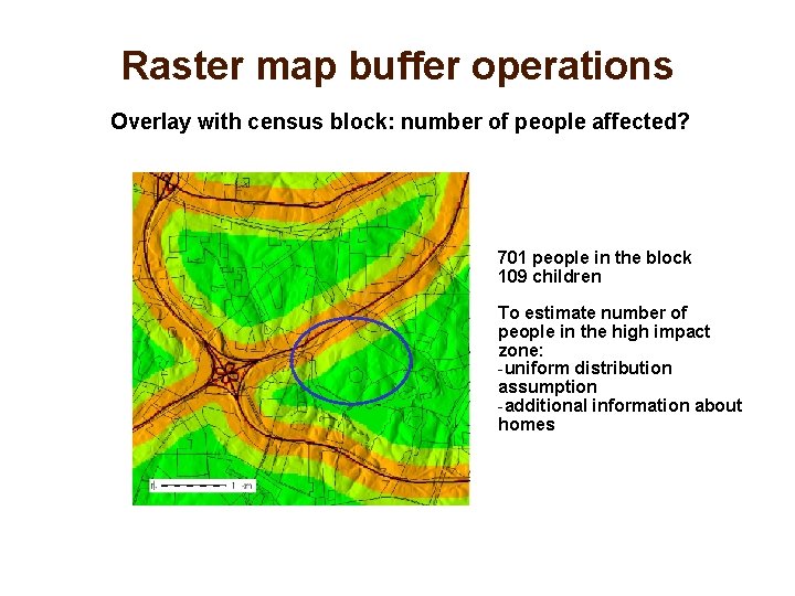
Raster map buffer operations Overlay with census block: number of people affected? 701 people in the block 109 children To estimate number of people in the high impact zone: -uniform distribution assumption -additional information about homes

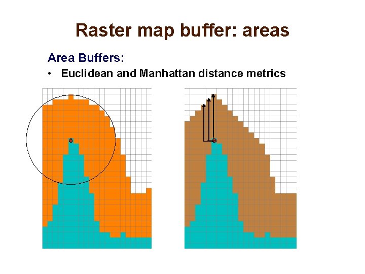
Raster map buffer: areas Area Buffers: • Euclidean and Manhattan distance metrics

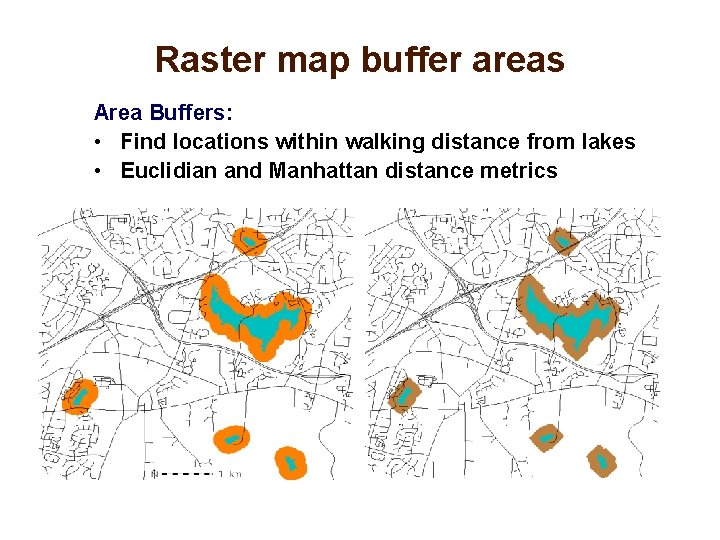
Raster map buffer areas Area Buffers: • Find locations within walking distance from lakes • Euclidian and Manhattan distance metrics

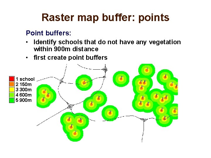
Raster map buffer: points Point buffers: • Identify schools that do not have any vegetation within 900 m distance • first create point buffers 1 school 2 150 m 3 300 m 4 600 m 5 900 m

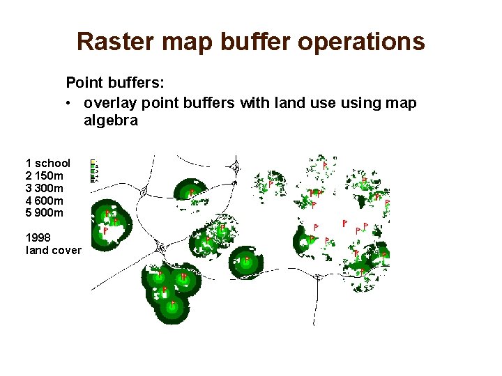
Raster map buffer operations Point buffers: • overlay point buffers with land use using map algebra 1 school 2 150 m 3 300 m 4 600 m 5 900 m 1998 land cover

Cost surfaces Cumulative (accumulated) cost surface: raster representation of cumulative cost of reaching the target point(s) from any location in the given region. Input cost map value assigned to a cell represents cost of traversing that cell, e. g. time estimated from: – inverse of speed limit for driving, – slope and/or vegetation density for walking

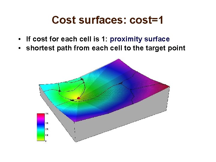
Cost surfaces: cost=1 • If cost for each cell is 1: proximity surface • shortest path from each cell to the target point

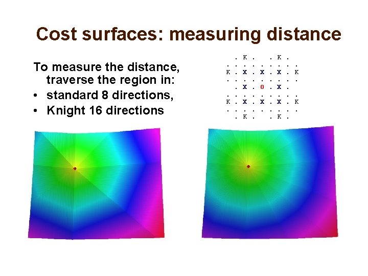
Cost surfaces: measuring distance To measure the distance, traverse the region in: • standard 8 directions, • Knight 16 directions . K. . . K. X. X. X. K . . X. O. X. . K. X. X. X. K . . K.

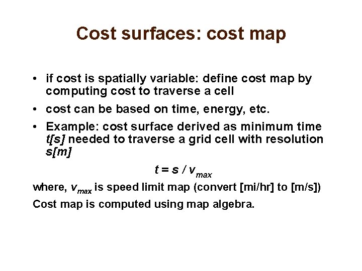
Cost surfaces: cost map • if cost is spatially variable: define cost map by computing cost to traverse a cell • cost can be based on time, energy, etc. • Example: cost surface derived as minimum time t[s] needed to traverse a grid cell with resolution s[m] t = s / vmax where, vmax is speed limit map (convert [mi/hr] to [m/s]) Cost map is computed using map algebra.

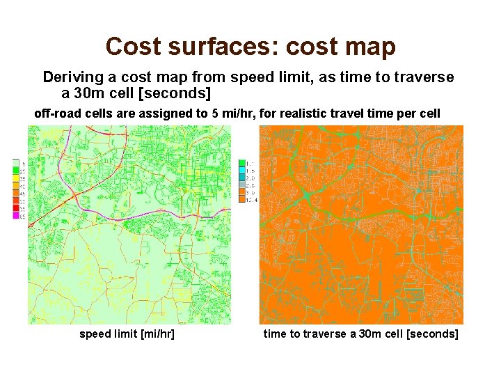
Cost surfaces: cost map Deriving a cost map from speed limit, as time to traverse a 30 m cell [seconds] off-road cells are assigned to 5 mi/hr, for realistic travel time per cell speed limit [mi/hr] time to traverse a 30 m cell [seconds]

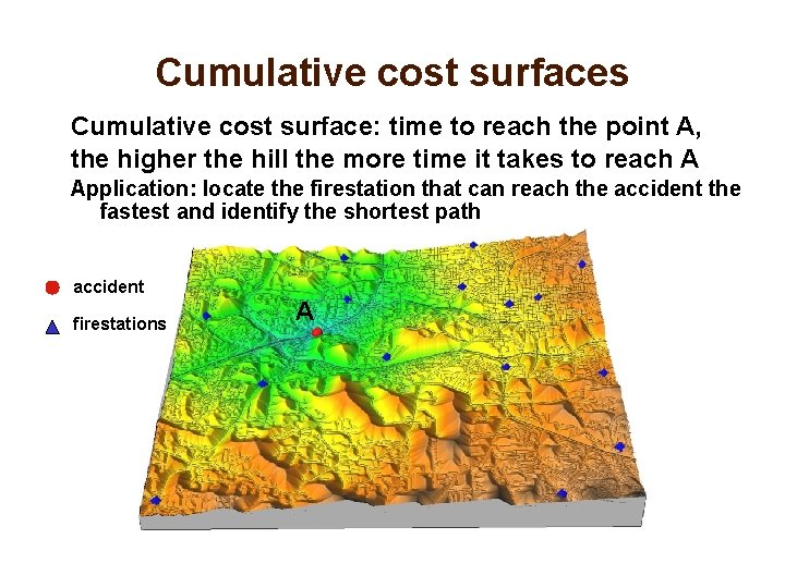
Cumulative cost surfaces Cumulative cost surface: time to reach the point A, the higher the hill the more time it takes to reach A Application: locate the firestation that can reach the accident the fastest and identify the shortest path accident firestations A

Least cost path • using the cumulative cost surface, find the least cost (fastest) path to the target point • least cost path (LCP) follows the steepest slope line, equivalent to flow routing with terrain replaced by cost surface • depending on algorithm used for flow routing depressions or flats in cost surface may lead to wrong results • save the directions used for creating the cumulative cost surface as back-link and compute LCP as tracked path

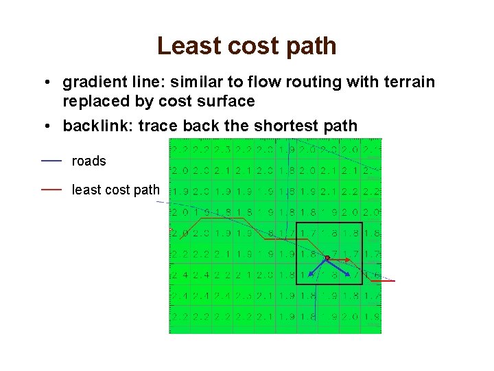
Least cost path • gradient line: similar to flow routing with terrain replaced by cost surface • backlink: trace back the shortest path roads least cost path

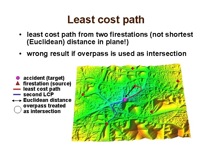
Least cost path • least cost path from two firestations (not shortest (Euclidean) distance in plane!) • wrong result if overpass is used as intersection accident (target) firestation (source) least cost path second LCP Euclidean distance overpass treated as intersection

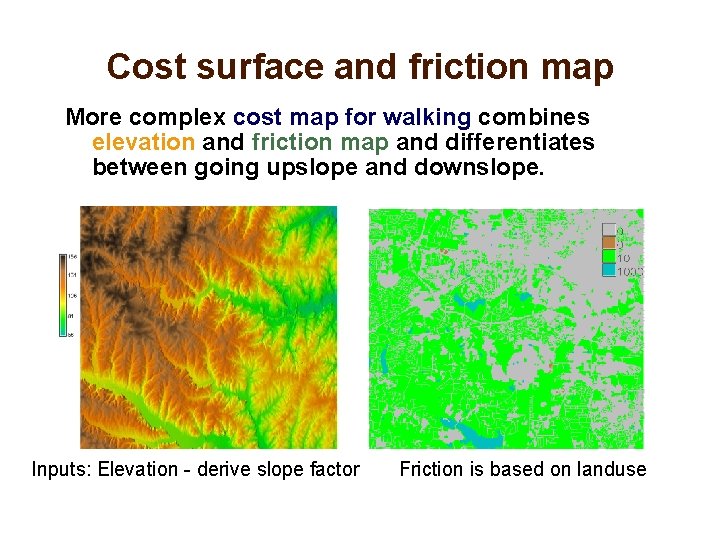
Cost surface and friction map More complex cost map for walking combines elevation and friction map and differentiates between going upslope and downslope. Inputs: Elevation - derive slope factor Friction is based on landuse

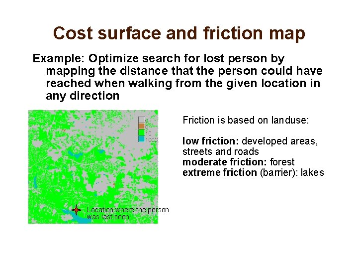
Cost surface and friction map Example: Optimize search for lost person by mapping the distance that the person could have reached when walking from the given location in any direction Friction is based on landuse: low friction: developed areas, streets and roads moderate friction: forest extreme friction (barrier): lakes Location where the person was last seen

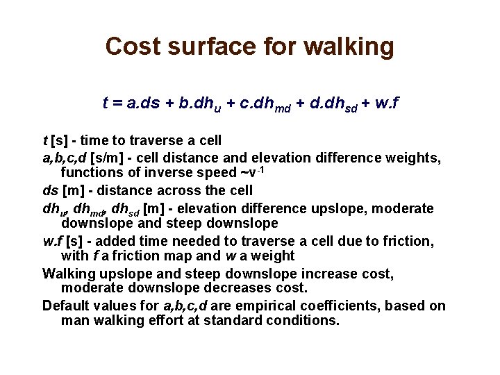
Cost surface for walking t = a. ds + b. dhu + c. dhmd + d. dhsd + w. f t [s] - time to traverse a cell a, b, c, d [s/m] - cell distance and elevation difference weights, functions of inverse speed ~v-1 ds [m] - distance across the cell dhu, dhmd, dhsd [m] - elevation difference upslope, moderate downslope and steep downslope w. f [s] - added time needed to traverse a cell due to friction, with f a friction map and w a weight Walking upslope and steep downslope increase cost, moderate downslope decreases cost. Default values for a, b, c, d are empirical coefficients, based on man walking effort at standard conditions.

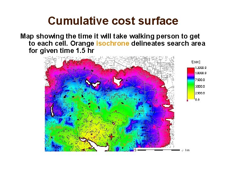
Cumulative cost surface Map showing the time it will take walking person to get to each cell. Orange isochrone delineates search area for given time 1. 5 hr t[sec]

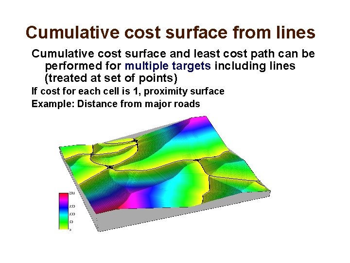
Cumulative cost surface from lines Cumulative cost surface and least cost path can be performed for multiple targets including lines (treated at set of points) If cost for each cell is 1, proximity surface Example: Distance from major roads

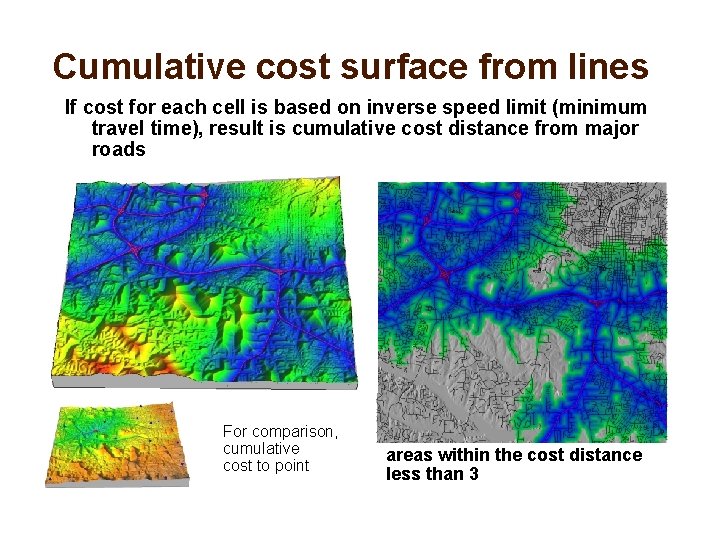
Cumulative cost surface from lines If cost for each cell is based on inverse speed limit (minimum travel time), result is cumulative cost distance from major roads For comparison, cumulative cost to point areas within the cost distance less than 3

Summary and references • measuring distance – http: //en. wikipedia. org/wiki/Great_circle • buffers – Neteler ch. 5. 4. 2 • cost surfaces, least cost path – Neteler ch. 5. 4. 3 – de. Smith, Goodchild, and Longley: Geospatial Analysis, http: //www. spatialanalysisonline. com/output/html/Accumulatedcostsurfacesandleastcostpaths. html – Berry, J. K. Beyond mapping III http: //www. innovativegis. com/basis/Map. Analysis/Default. htm