Geometric Algorithms Suman Sourav Paramasiven Appavoo Anuja Meetoo

Geometric Algorithms Suman Sourav Paramasiven Appavoo Anuja Meetoo Appavoo Li Jing Lu Bingxin Suhendry Effendy Dumitrel Loghin

Introduction & Motivation Suman Sourav

Introduction • Computational geometry is a branch of computer science devoted to the study of algorithms which can be stated in terms of geometry. • Deep connections with classical mathematics and theoretical computer science on the one hand, and many ties with applications on the other. • Focus is on discrete nature of geometric problems as opposed to continuous issues.

Introduction • • • Any problem that is to be solved using a digital computer has to be discrete in form. For CG techniques to be applied to areas that involves continuous issues, discrete approximations to continuous curves or surfaces are needed. People deal more with straight or flat objects or simple curved objects, than with high degree algebraic curves.

Introduction • • Programming in CG is a little difficult. Libraries like LEDA and CGAL implement various data structures and geometric algorithms. CG algorithms suffer from the curse of degeneracies. So, certain simplifying assumptions at times like no three points are collinear, no four points are cocircular, etc are needed to be made.

Motivation & Application There are many areas that give rise to geometric problems. • • Computer graphics Computer vision and image processing Robotics Computer-aided designing (CAD) Geographic information systems (GIS) Telecommunication VLSI design (chip layout)

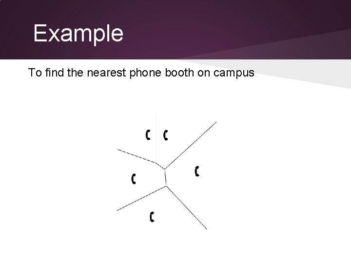
Example To find the nearest phone booth on campus

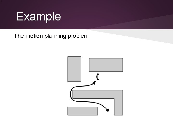
Example The motion planning problem

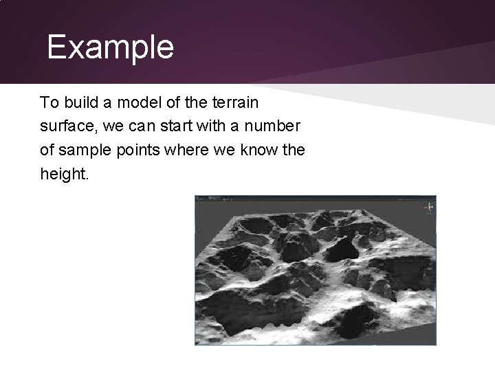
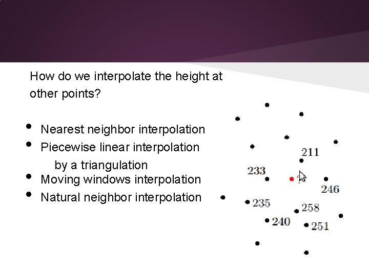
Example To build a model of the terrain surface, we can start with a number of sample points where we know the height.

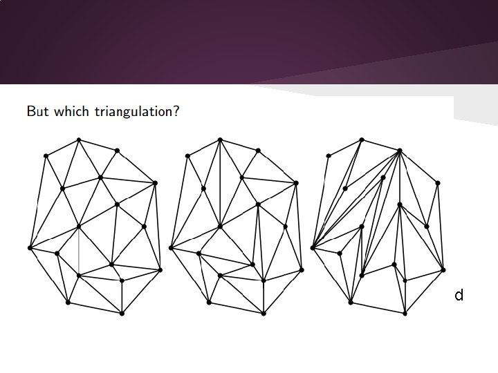
How do we interpolate the height at other points? • • Nearest neighbor interpolation Piecewise linear interpolation by a triangulation Moving windows interpolation Natural neighbor interpolation

For interpolation, it is good if triangles are not long and skinny.

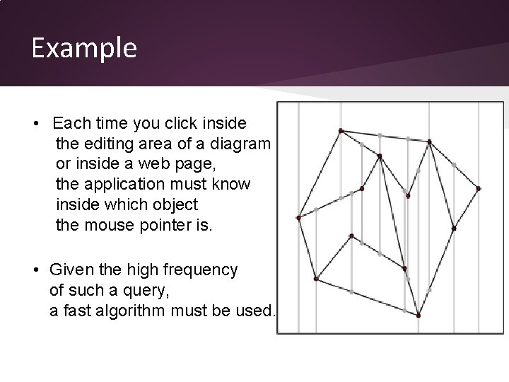
Example • Each time you click inside the editing area of a diagram or inside a web page, the application must know inside which object the mouse pointer is. • Given the high frequency of such a query, a fast algorithm must be used.

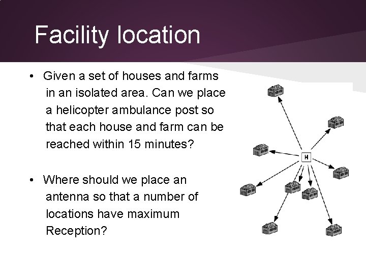
Facility location • Given a set of houses and farms in an isolated area. Can we place a helicopter ambulance post so that each house and farm can be reached within 15 minutes? • Where should we place an antenna so that a number of locations have maximum Reception?

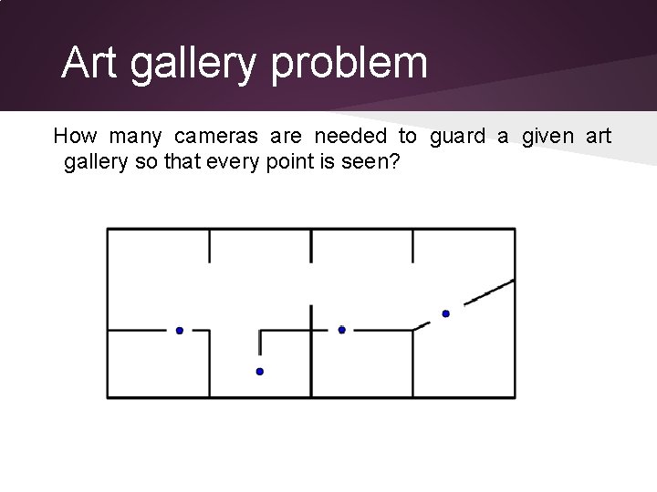
Art gallery problem How many cameras are needed to guard a given art gallery so that every point is seen?

A Real Life Application

Voronoi diagram - Properties - Construction methods Fortune’s Algorithm - How does it work? - Implementation aspects - Data structures - Pseudocode - Complexity (time & space) Paramasiven Appavoo & Anuja Meetoo Appavoo

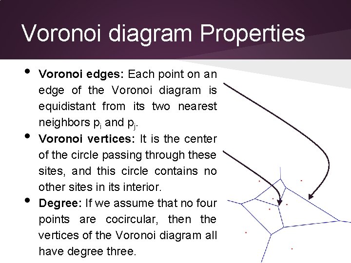
Voronoi diagram Properties • • • Voronoi edges: Each point on an edge of the Voronoi diagram is equidistant from its two nearest neighbors pi and pj. Voronoi vertices: It is the center of the circle passing through these sites, and this circle contains no other sites in its interior. Degree: If we assume that no four points are cocircular, then the vertices of the Voronoi diagram all have degree three.

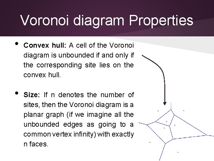
Voronoi diagram Properties • • Convex hull: A cell of the Voronoi diagram is unbounded if and only if the corresponding site lies on the convex hull. Size: If n denotes the number of sites, then the Voronoi diagram is a planar graph (if we imagine all the unbounded edges as going to a common vertex infinity) with exactly n faces.

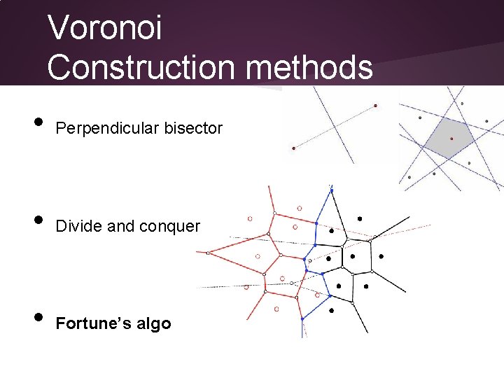
Voronoi Construction methods • Perpendicular bisector • Divide and conquer • Fortune’s algo

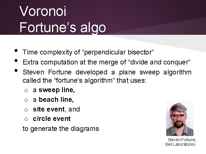
Voronoi Fortune’s algo • • • Time complexity of “perpendicular bisector” Extra computation at the merge of “divide and conquer” Steven Fortune developed a plane sweep algorithm called the “fortune’s algorithm” that uses: o a sweep line, o a beach line, o site event, and o circle event to generate the diagrams Steven Fortune, Bell Laboratories

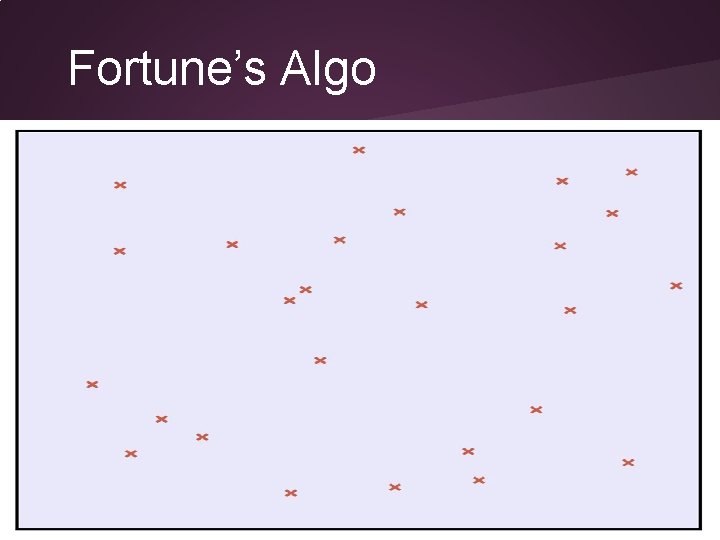
Fortune’s Algo

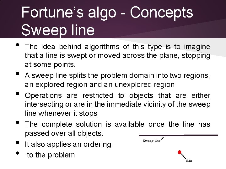
• • • Fortune’s algo - Concepts Sweep line The idea behind algorithms of this type is to imagine that a line is swept or moved across the plane, stopping at some points. A sweep line splits the problem domain into two regions, an explored region and an unexplored region Operations are restricted to objects that are either intersecting or are in the immediate vicinity of the sweep line whenever it stops The complete solution is available once the line has passed over all objects. It also applies an ordering to the problem

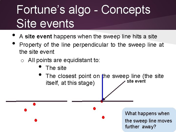
• • Fortune’s algo - Concepts Site events A site event happens when the sweep line hits a site Property of the line perpendicular to the sweep line at the site event o All points are equidistant to: The site The closest point on the sweep line (the site event itself, at this stage) • • What happens when the sweep line moves further away?

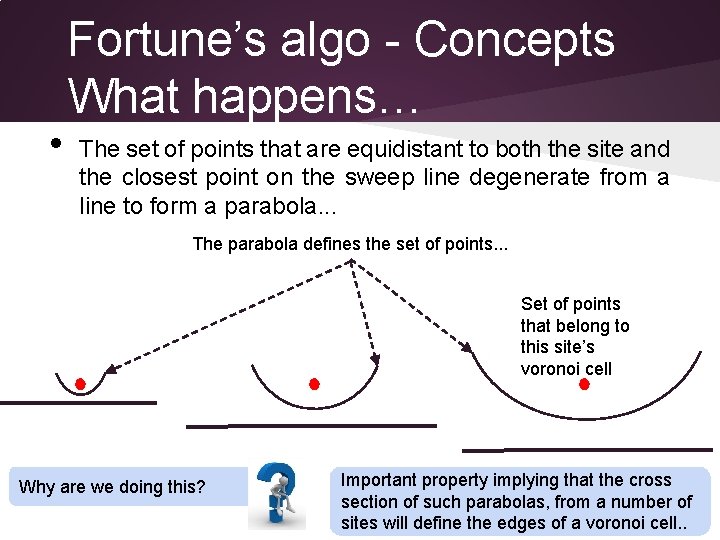
• Fortune’s algo - Concepts What happens… The set of points that are equidistant to both the site and the closest point on the sweep line degenerate from a line to form a parabola. . . The parabola defines the set of points. . . Set of points that belong to this site’s voronoi cell Why are we doing this? Important property implying that the cross section of such parabolas, from a number of sites will define the edges of a voronoi cell. .

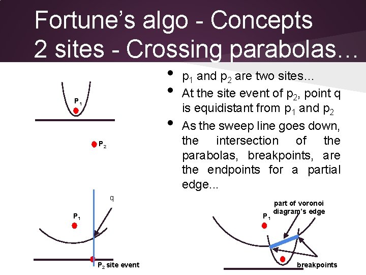
Fortune’s algo - Concepts 2 sites - Crossing parabolas… • • P 1 • P 2 p 1 and p 2 are two sites… At the site event of p 2, point q is equidistant from p 1 and p 2 As the sweep line goes down, the intersection of the parabolas, breakpoints, are the endpoints for a partial edge. . . q P 1 P 2 site event part of voronoi diagram’s edge breakpoints

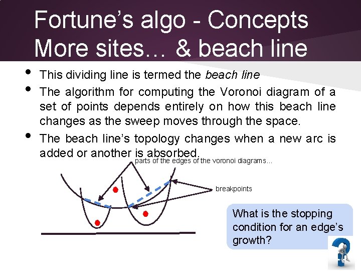
• • • Fortune’s algo - Concepts More sites… & beach line This dividing line is termed the beach line The algorithm for computing the Voronoi diagram of a set of points depends entirely on how this beach line changes as the sweep moves through the space. The beach line’s topology changes when a new arc is added or another is absorbed. parts of the edges of the voronoi diagrams. . . breakpoints What is the stopping condition for an edge’s growth?

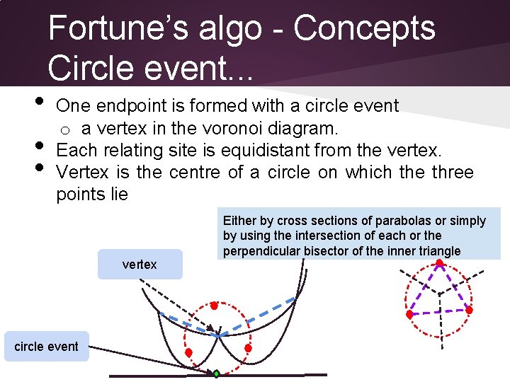
• • • Fortune’s algo - Concepts Circle event. . . One endpoint is formed with a circle event o a vertex in the voronoi diagram. Each relating site is equidistant from the vertex. Vertex is the centre of a circle on which the three points lie vertex circle event Either by cross sections of parabolas or simply by using the intersection of each or the perpendicular bisector of the inner triangle

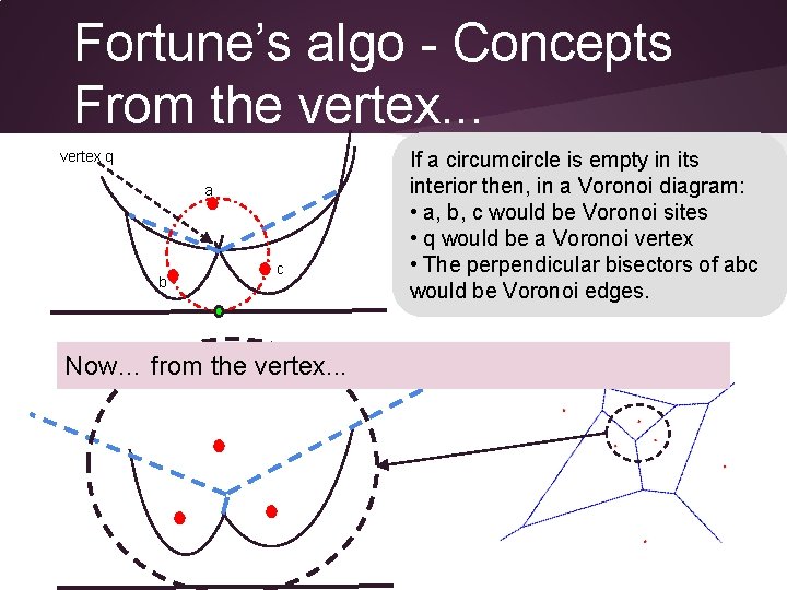
Fortune’s algo - Concepts From the vertex. . . vertex q a b c Now… from the vertex. . . If a circumcircle is empty in its interior then, in a Voronoi diagram: • a, b, c would be Voronoi sites • q would be a Voronoi vertex • The perpendicular bisectors of abc would be Voronoi edges.

Fortune’s algo Implementation Aspects. . . • • Parabolas defining beach line not computed as sweep line moves through the problem space o Computationally expensive and unnecessary o Calculations required only when the beach line changes topology § Site events § Circle events Sweep line makes discrete steps, rather than a continuous sweep

Fortune’s algo Data Structures • • • Priority queue o State of sweep line o Indicates when topology of beach line can change § Site events § Circle events Doubly connected edge list (DCEL) o State of Voronoi diagram o Stores § Vertex records § Edge records § Face records Balanced binary search tree ( AVL or red-black tree) o State of beach line

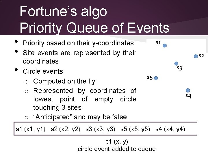
• • • Fortune’s algo Priority Queue of Events Priority based on their y-coordinates Site events are represented by their coordinates Circle events o Computed on the fly o Represented by coordinates of lowest point of empty circle touching 3 sites o “Anticipated” and may be false s 1 (x 1, y 1) s 2 (x 2, y 2) s 3 (x 3, y 3) s 5 (x 5, y 5) s 4 (x 4, y 4) c 1 (x, y) circle event added to queue

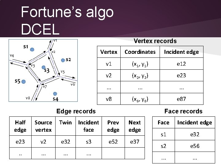
Fortune’s algo DCEL Vertex records Vertex Coordinates Incident edge v 1 (x 1, y 1) e 12 v 2 (x 2, y 2) e 23 . . v 8 (x 8, y 8) e 87 Edge records Half edge Source vertex Twin e 23 v 2 . . . Face records Incident face Prev edge Next edge e 32 s 3 e 52 e 37 . . . Face Incident edge s 1 e 32 s 2 e 56 . . .

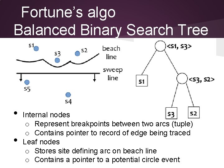
Fortune’s algo Balanced Binary Search Tree • • Internal nodes o Represent breakpoints between two arcs (tuple) o Contains pointer to record of edge being traced Leaf nodes o Stores site defining arc on beach line o Contains a pointer to a potential circle event

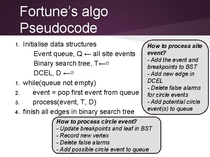
Fortune’s algo Pseudocode 1. 2. 3. 4. Initialise data structures Event queue, Q ← all site events Binary search tree, T←∅ DCEL, D ←∅ while(queue not empty) event = pop first event from queue process(event, T, D) finish all edges in binary search tree How to process site event? - Add the event and breakpoints to BST - Add new edge in DCEL - Delete false alarms for circle events - Add potential circle event(s) to queue How to process circle event? - Update breakpoints and leaf in BST - Record new vertex - Delete false alarms - Add possible circle event to queue

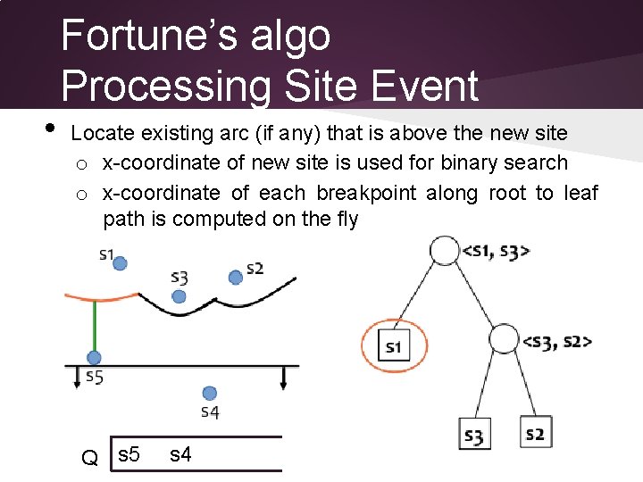
• Fortune’s algo Processing Site Event Locate existing arc (if any) that is above the new site o x-coordinate of new site is used for binary search o x-coordinate of each breakpoint along root to leaf path is computed on the fly Q s 5 s 4

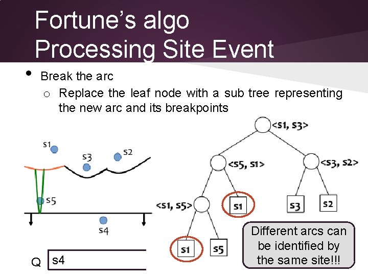
• Fortune’s algo Processing Site Event Break the arc o Replace the leaf node with a sub tree representing the new arc and its breakpoints Q s 4 Different arcs can be identified by the same site!!!

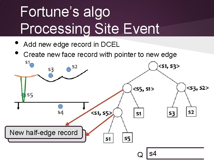
• • Fortune’s algo Processing Site Event Add new edge record in DCEL Create new face record with pointer to new edge New half-edge record Q s 4

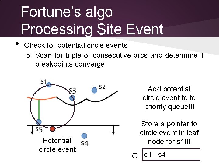
• Fortune’s algo Processing Site Event Check for potential circle events o Scan for triple of consecutive arcs and determine if breakpoints converge Add potential circle event to to priority queue!!! Potential circle event Store a pointer to circle event in leaf node for s 1!!! Q c 1 s 4

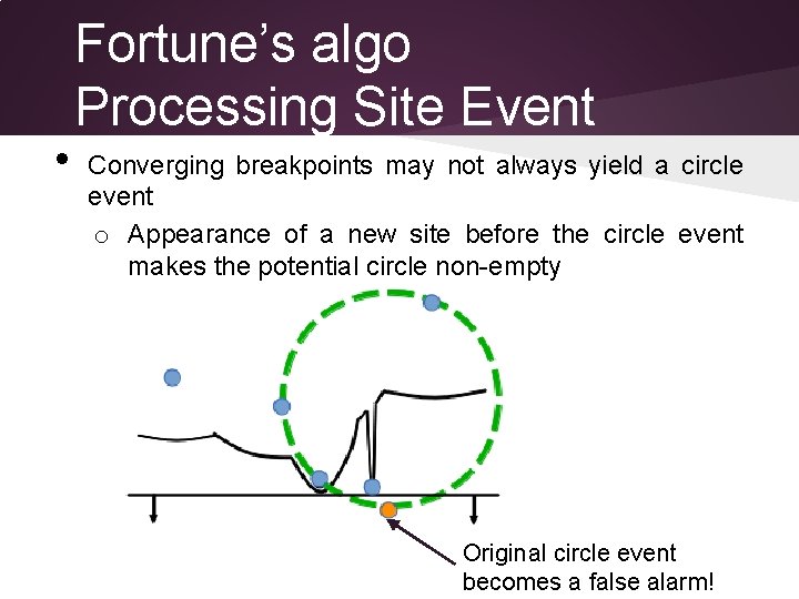
• Fortune’s algo Processing Site Event Converging breakpoints may not always yield a circle event o Appearance of a new site before the circle event makes the potential circle non-empty Original circle event becomes a false alarm!

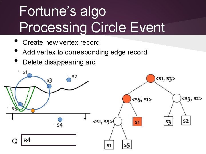
• • • Fortune’s algo Processing Circle Event Create new vertex record Add vertex to corresponding edge record Delete disappearing arc Q s 4

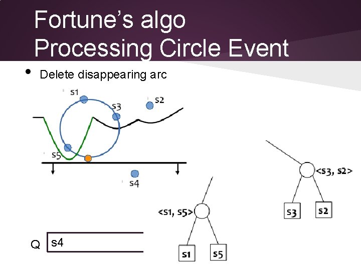
• Fortune’s algo Processing Circle Event Delete disappearing arc Q s 4

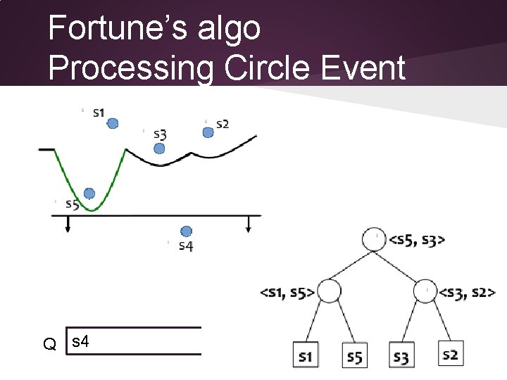
Fortune’s algo Processing Circle Event Q s 4

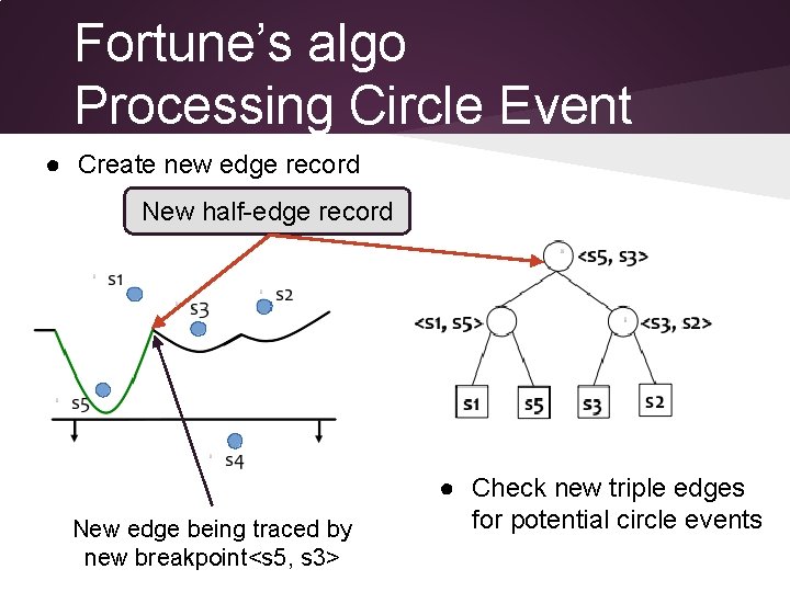
Fortune’s algo Processing Circle Event ● Create new edge record New half-edge record New edge being traced by new breakpoint<s 5, s 3> ● Check new triple edges for potential circle events

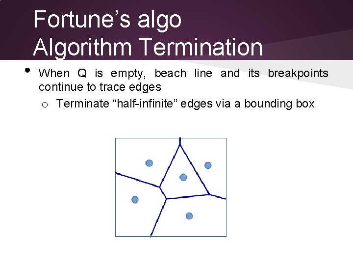
• Fortune’s algo Algorithm Termination When Q is empty, beach line and its breakpoints continue to trace edges o Terminate “half-infinite” edges via a bounding box

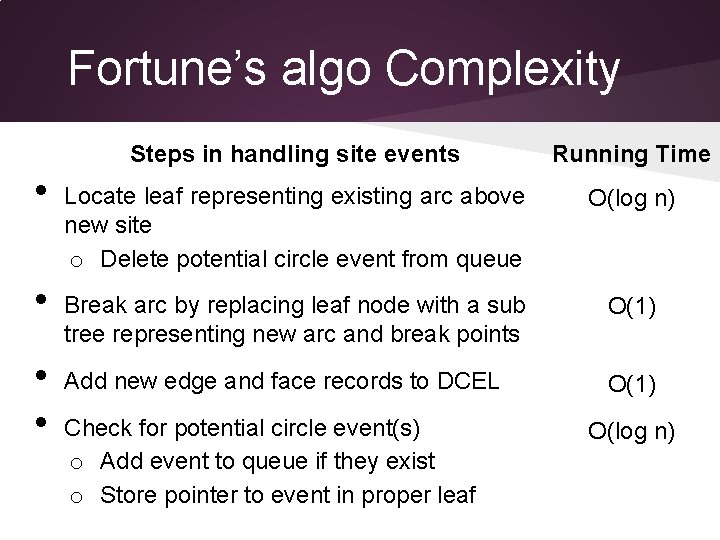
Fortune’s algo Complexity • • Steps in handling site events Running Time Locate leaf representing existing arc above new site o Delete potential circle event from queue O(log n) Break arc by replacing leaf node with a sub tree representing new arc and break points O(1) Add new edge and face records to DCEL O(1) Check for potential circle event(s) o Add event to queue if they exist o Store pointer to event in proper leaf O(log n)

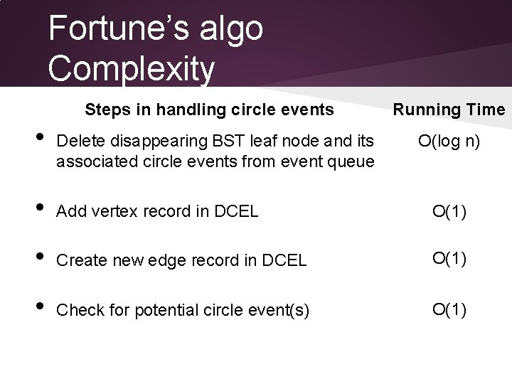
Fortune’s algo Complexity Steps in handling circle events • Delete disappearing BST leaf node and its associated circle events from event queue Running Time O(log n) • Add vertex record in DCEL O(1) • Create new edge record in DCEL O(1) • Check for potential circle event(s) O(1)

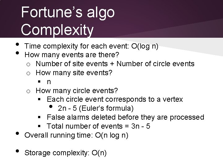
• • Fortune’s algo Complexity Time complexity for each event: O(log n) How many events are there? o Number of site events + Number of circle events o How many site events? § n o How many circle events? § Each circle event corresponds to a vertex 2 n - 5 (Euler’s formula) § False alarms deleted before they are processed § Total number of events = 3 n - 5 Overall running time: O(n log n) • • • Storage complexity: O(n)

Delaunay Triangulation • Delaunay and Voronoi • Delaunay properties • Randomized Algorithm - Idea - Implementation aspects - Pseudocode - Data structure - Complexity (time & space) Li Jing & Lu Bingxin

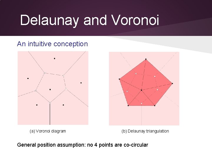
Delaunay and Voronoi An intuitive conception (a) Voronoi diagram (b) Delaunay triangulation General position assumption: no 4 points are co-circular

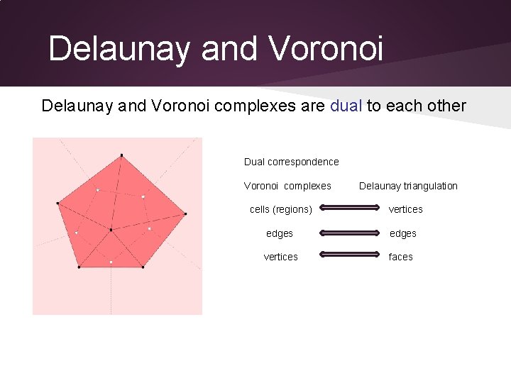
Delaunay and Voronoi complexes are dual to each other Dual correspondence Voronoi complexes Delaunay triangulation cells (regions) vertices edges vertices faces

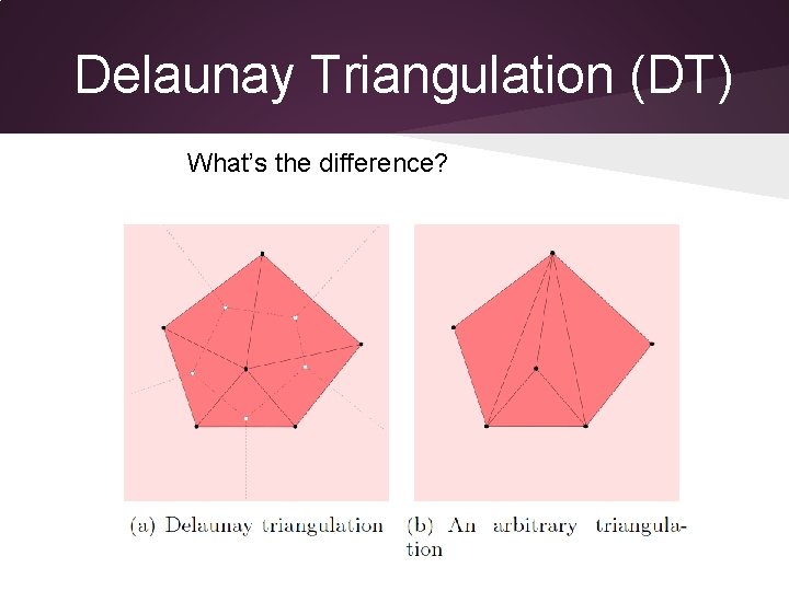
Delaunay Triangulation (DT) What’s the difference?

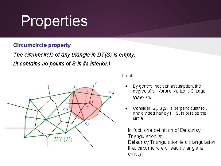
Properties Circumcircle property The circumcircle of any triangle in DT{S) is empty. (It contains no points of S in its interior. ) Proof ● By general position assumption, the degree of all Voronoi vertex is 3, edge vu exists ● Consider S 4, S 1 S 4 is perpendicular to l and divided half by l . S 4 is outside the circle In fact, one definition of Delaunay Triangulation is: Delaunay Triangulation is a triangulation that circumcircle of each triangle is empty.

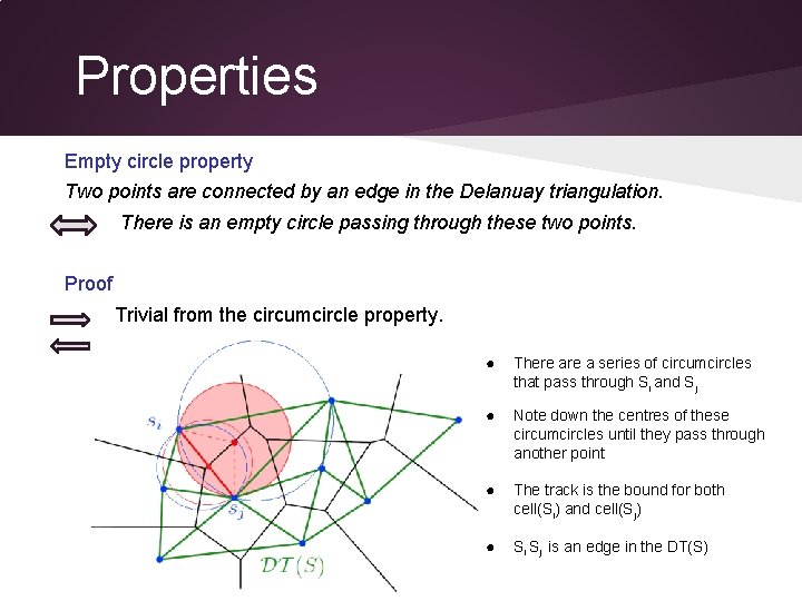
Properties Empty circle property Two points are connected by an edge in the Delanuay triangulation. There is an empty circle passing through these two points. Proof Trivial from the circumcircle property. ● There a series of circumcircles that pass through Si and Sj ● Note down the centres of these circumcircles until they pass through another point ● The track is the bound for both cell(Si) and cell(Sj) ● Si Sj is an edge in the DT(S)

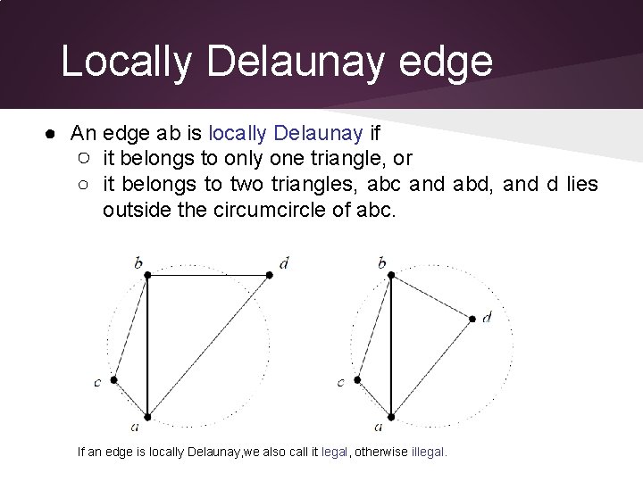
Locally Delaunay edge ● An edge ab is locally Delaunay if ○ it belongs to only one triangle, or ○ it belongs to two triangles, abc and abd, and d lies outside the circumcircle of abc. If an edge is locally Delaunay, we also call it legal, otherwise illegal.

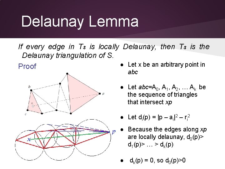
Delaunay Lemma If every edge in Ts is locally Delaunay, then Ts is the Delaunay triangulation of S. ● Let x be an arbitrary point in Proof abc ● Let abc=Α 0, A 1, A 2, … Ak be the sequence of triangles that intersect xp ● Let di(p) = |p – ai|2 – ri 2 ● Because the edges along xp are locally delaunay, d 0(p)> d 1(p)> … > dk(p) ● dk(p) = 0, so d 0(p)>0

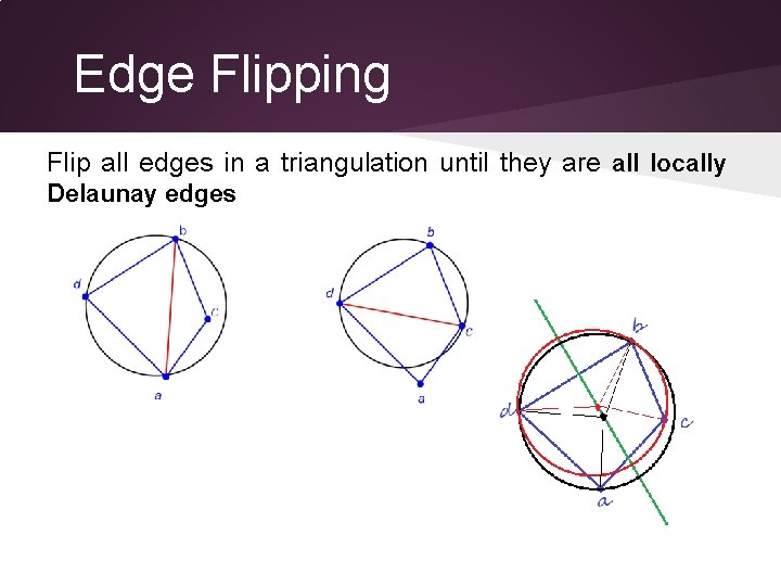
Edge Flipping Flip all edges in a triangulation until they are all locally Delaunay edges

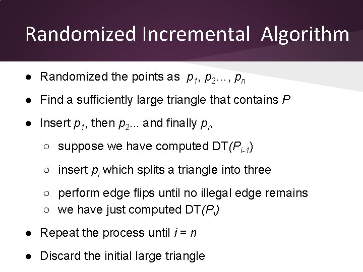
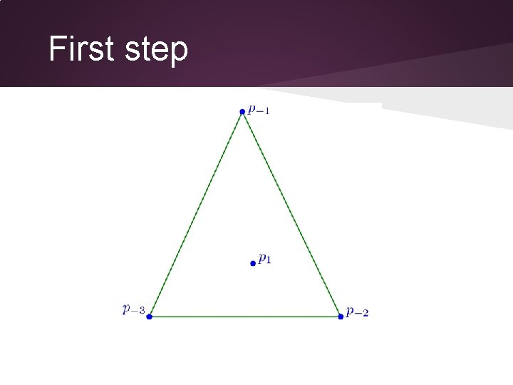
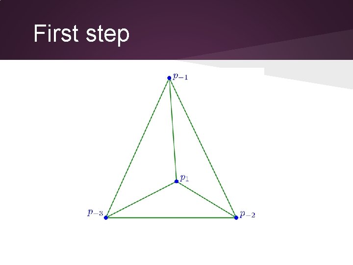
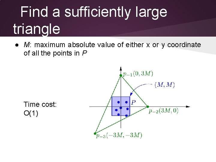
Randomized Incremental Algorithm ● Randomized the points as p 1, p 2…, pn ● Find a sufficiently large triangle that contains P ● Insert p 1, then p 2. . . and finally pn ○ suppose we have computed DT(Pi-1) ○ insert pi which splits a triangle into three ○ perform edge flips until no illegal edge remains ○ we have just computed DT(Pi) ● Repeat the process until i = n ● Discard the initial large triangle

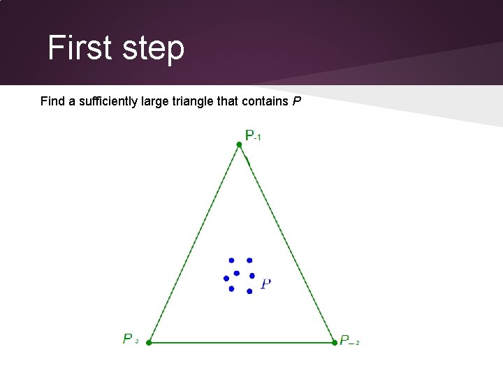
First step Find a sufficiently large triangle that contains P

First step

First step

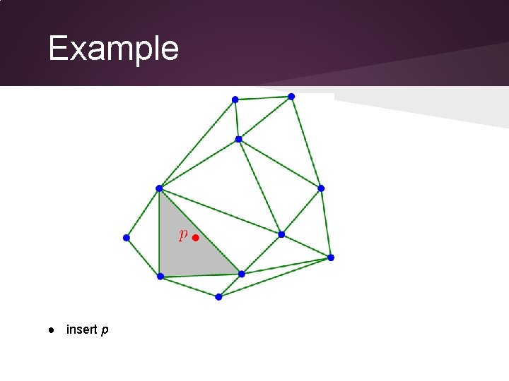
Example ● insert p

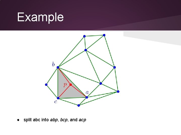
Example ● split abc into abp, bcp, and acp

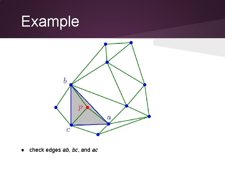
Example ● check edges ab, bc, and ac

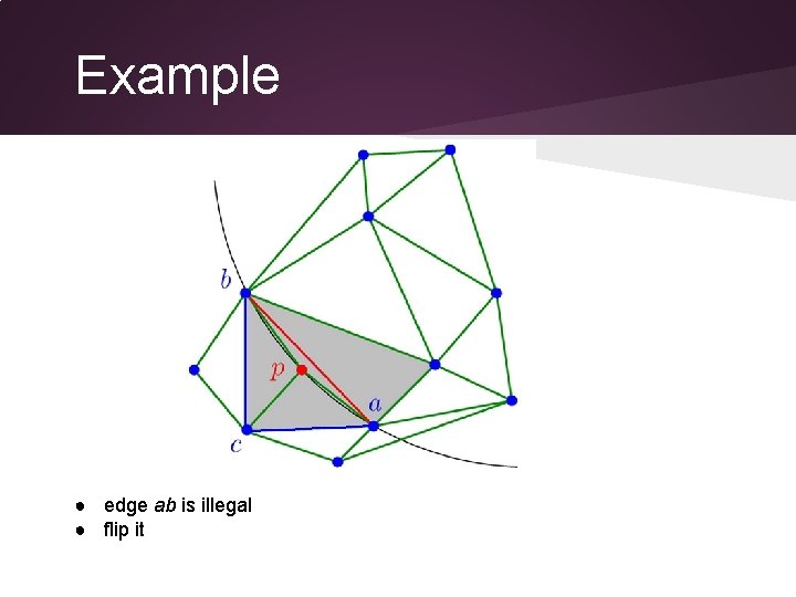
Example ● edge ab is illegal ● flip it

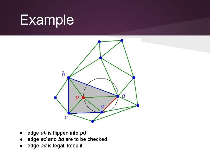
Example ● edge ab is flipped into pd ● edge ad and bd are to be checked ● edge ad is legal, keep it

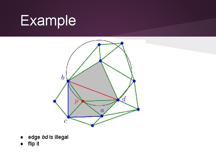
Example ● edge bd is illegal ● flip it

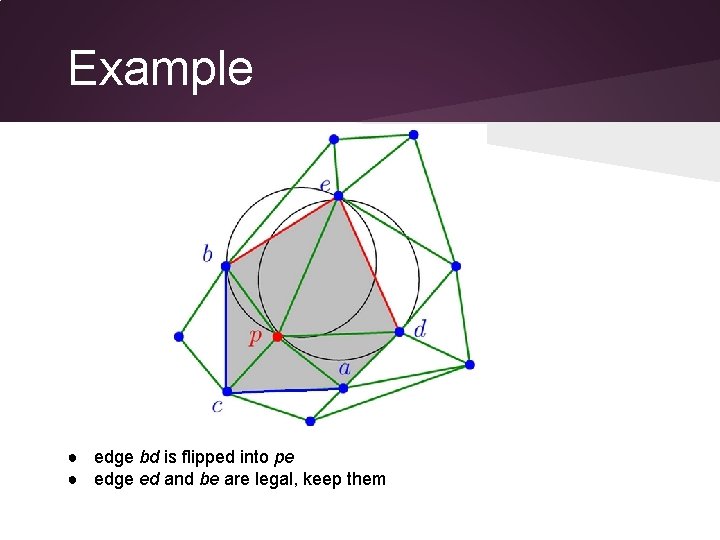
Example ● edge bd is flipped into pe ● edge ed and be are legal, keep them

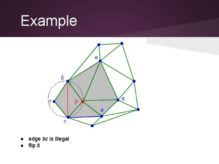
Example ● edge bc is illegal ● flip it

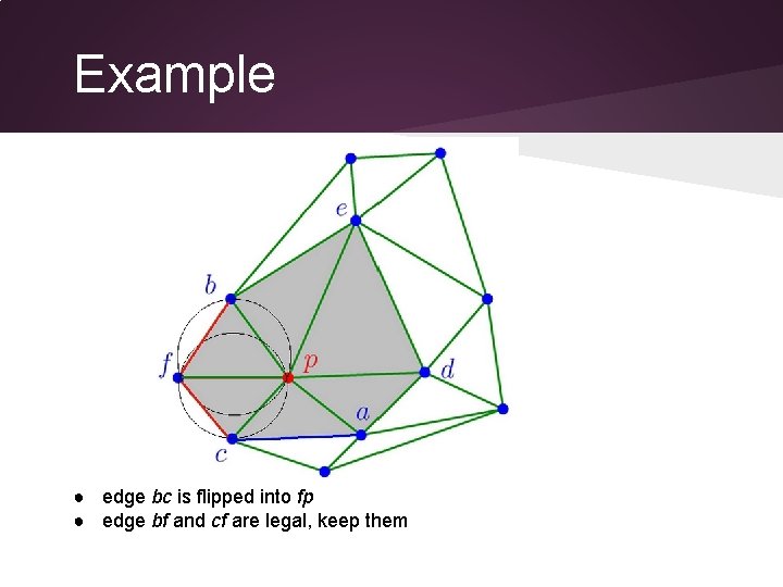
Example ● edge bc is flipped into fp ● edge bf and cf are legal, keep them

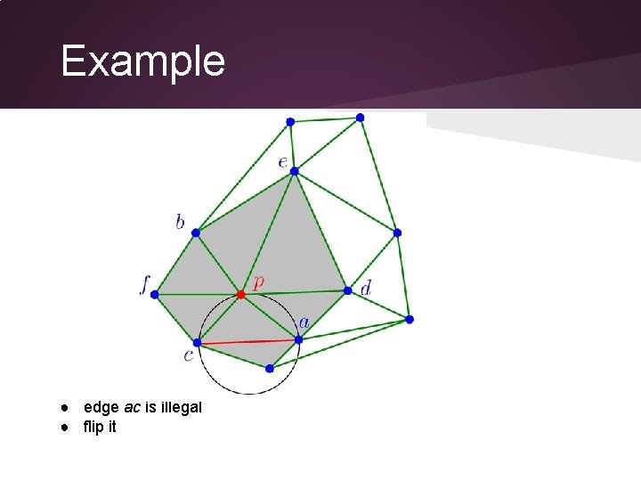
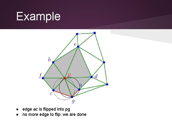
Example ● edge ac is illegal ● flip it

Example ● edge ac is flipped into pg ● no more edge to flip: we are done

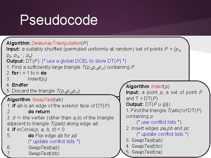
Pseudocode Algorithm Delaunay. Triangulation(P) Input: a suitably shuffled (permuted uniformly at random) set of points P = (p 1, p 2, p 3, . ⋯, pn) Output: DT(P) (* use a global DCEL to store DT(P) *) 1. Find a sufficiently large triangle T(p-3 p-2 p-1) containing P 2. for i = 1 to n do 3. Insert(pi) 4. Endfor Algorithm Insert(p) 5. Discard the triangle T(p-3 p-2 p-1) Input: a point p, a set of point P and T = DT(P) Algorithm Swap. Test(ab) Output: DT(P u {p}) 1. if ab is an edge of the exterior face of DT(P) 1. Find the triangle T(abc) of DT(P) 2. do return containing p 3. d <- the vertex (other than a, b) of the triangle (* use conflict lists *) adjacent to triangle T(pab) along edge ab 2. Insert edges pa, pb and pc 4. if in. Circle(p, a, b, d) < 0 (* update conflict lists *) 5. do Flip edge ab for pd 3. Swap. Test(ab) (* update conflict lists *) 4. Swap. Test(bc) 6. Swap. Test(ad) 5. Swap. Test(ca) 7. Swap. Test(db)

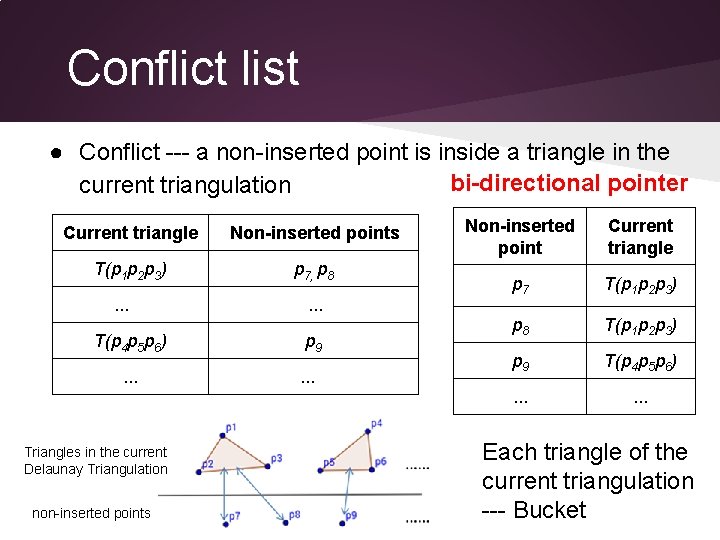
Conflict list ● Conflict --- a non-inserted point is inside a triangle in the bi-directional pointer current triangulation Current triangle Non-inserted points T(p 1 p 2 p 3) p 7, p 8 . . . T(p 4 p 5 p 6). . . Triangles in the current Delaunay Triangulation non-inserted points . . . p 9 . . . Non-inserted point Current triangle p 7 T(p 1 p 2 p 3) p 8 T(p 1 p 2 p 3) p 9 T(p 4 p 5 p 6) . . . Each triangle of the current triangulation --- Bucket

Time complexity ● Major steps in the algorithm ○ Find a sufficiently large triangle ○ Find the triangle containing a non-inserted point ○ Update the triangulation ○ Update conflict lists

Find a sufficiently large triangle ● M: maximum absolute value of either x or y coordinate of all the points in P Time cost: O(1)

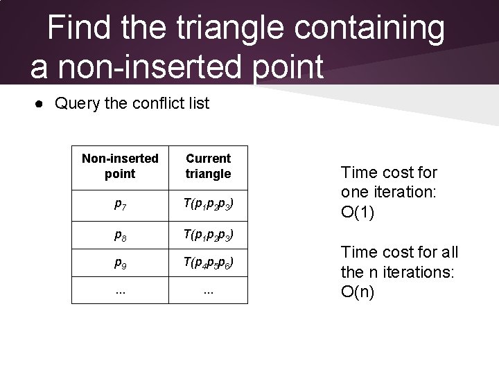
Find the triangle containing a non-inserted point ● Query the conflict list Non-inserted point Current triangle p 7 T(p 1 p 2 p 3) p 8 T(p 1 p 2 p 3) p 9 T(p 4 p 5 p 6) . . . Time cost for one iteration: O(1) Time cost for all the n iterations: O(n)

Backward analysis ● Imagine that the algorithm is run backwards starting from the delaunay triangulation we have at the end ● In analyzing the ith step, imagine that we are deleting one of the i points in the current triangulation and then update the triangulation ○ The work done in this case is the same as running the algorithm forward ○ Assume that each of the i points is equally likely to be deleted at the ith step, since the points were added randomly in the original algorithm

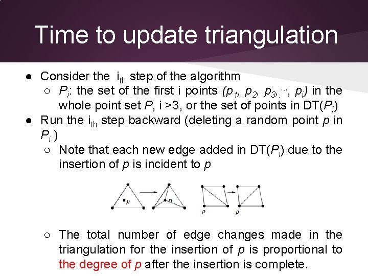
Time to update triangulation ● Consider the ith step of the algorithm ○ Pi: the set of the first i points (p 1, p 2, p 3, . ⋯, pi) in the whole point set P, i >3, or the set of points in DT(Pi) ● Run the ith step backward (deleting a random point p in Pi ) ○ Note that each new edge added in DT(Pi) due to the insertion of p is incident to p ○ The total number of edge changes made in the triangulation for the insertion of p is proportional to the degree of p after the insertion is complete.

Time to update triangulation ● The total degree of the vertices in Pi is less than 6 i ○ There at most 3 i edges in DT(Pi) (planar graph) ○ The sum of vertex degrees is twice the number of edges in a graph ● The expected degree of a random point in Pi is at most 6 ● The expected number of edge changes for inserting a random point p is O(1) ● Summing over all the n steps, the time for updating the triangulation is O(n)

Update conflict lists ● Each non-inserted point is assigned to a triangle/bucket ● For a non-inserted point, if the triangle which it lies within is destroyed, we have to find another new triangle containing this non-inserted point ● The expected time to update conflict lists ○ is the expected time to rebucket non-inserted points ○ is proportional to the expected number of noninserted points required to be rebucketed

Rebucket points ● Consider the ith step of the algorithm ○ Pi: the set of the first i points (p 1, p 2, p 3, ⋯, pi) in the whole point set P, i >3, or the set of points in DT(Pi) ○ PPi : the set of non-inserted points (pi+1, pi+2, pi+3, ⋯, p n) ● Run the ith step backward (deleting a random point in Pi) ○ some triangles in DT(Pi) are destroyed ○ some points in PPi are required to be rebucketed

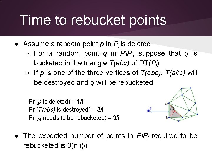
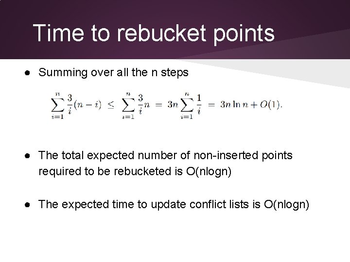
Time to rebucket points ● Assume a random point p in Pi is deleted ○ For a random point q in PPi, suppose that q is bucketed in the triangle T(abc) of DT(Pi) ○ If p is one of the three vertices of T(abc), T(abc) will be destroyed and q will be rebucketed Pr (p is deleted) = 1/i Pr (T(abc) is destroyed) = 3/i Pr (q needs to be rebucketed) = 3/i ● The expected number of points in PPi required to be rebucketed is 3(n-i)/i

Time to rebucket points ● Summing over all the n steps ● The total expected number of non-inserted points required to be rebucketed is O(nlogn) ● The expected time to update conflict lists is O(nlogn)

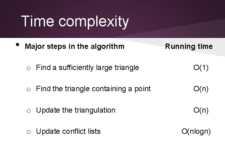
Time complexity • Major steps in the algorithm Running time o Find a sufficiently large triangle O(1) o Find the triangle containing a point O(n) o Update the triangulation O(n) o Update conflict lists O(nlogn)

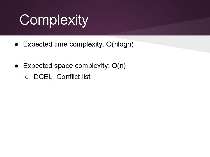
Complexity ● Expected time complexity: O(nlogn) ● Expected space complexity: O(n) ○ DCEL, Conflict list

Trapezoidal Decomposition Concepts Randomized Algorithm Motivation - Point Location Complexity Analysis Dumitrel Loghin & Suhendry Effendy

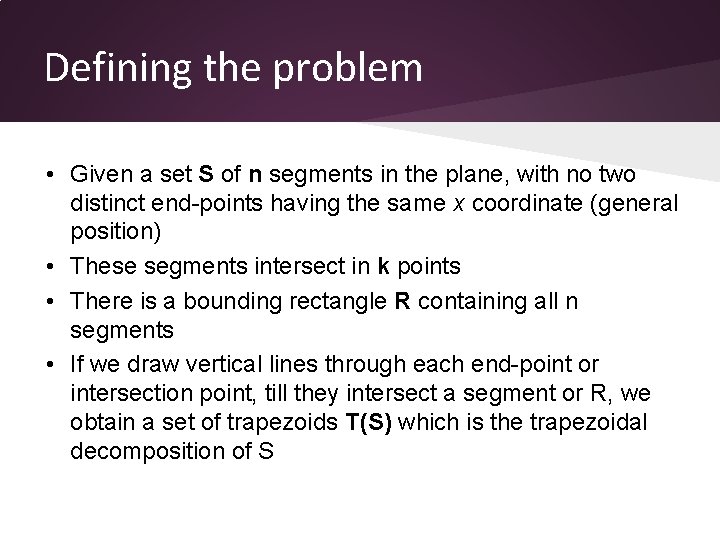
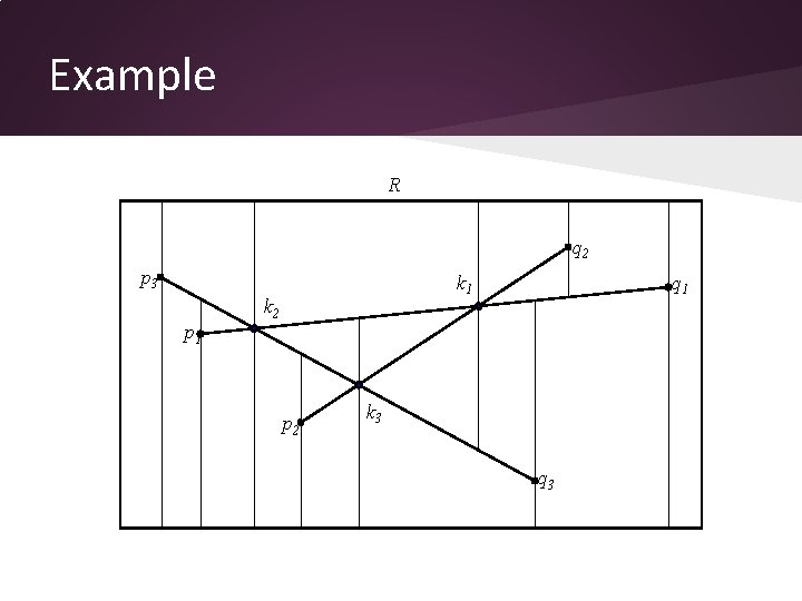
Defining the problem • Given a set S of n segments in the plane, with no two distinct end-points having the same x coordinate (general position) • These segments intersect in k points • There is a bounding rectangle R containing all n segments • If we draw vertical lines through each end-point or intersection point, till they intersect a segment or R, we obtain a set of trapezoids T(S) which is the trapezoidal decomposition of S

Example R q 2 p 3 p 1 k 2 p 2 q 1 k 3 q 3

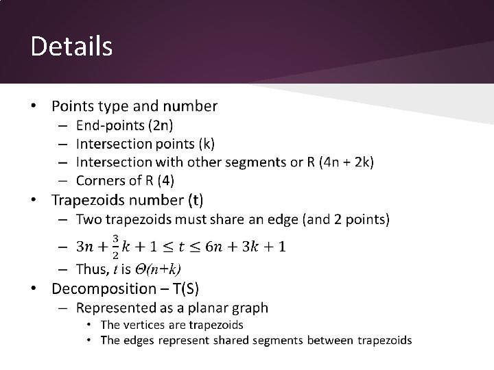
Details

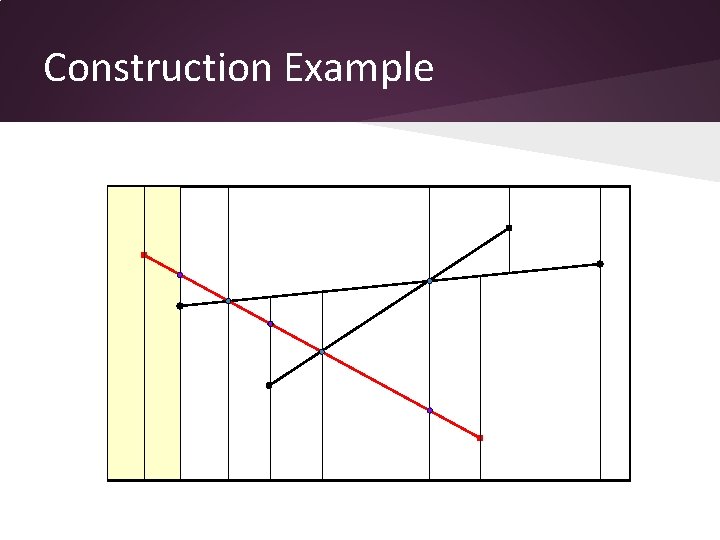
Construction Example

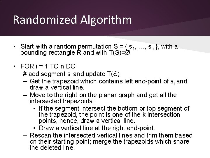
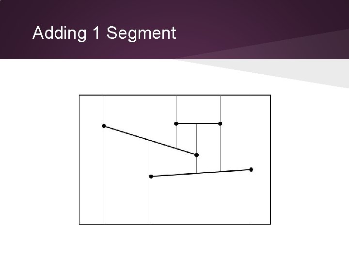
Randomized Algorithm • Start with a random permutation S = { s 1, …, sn }, with a bounding rectangle R and with T(S)=Ø • FOR i = 1 TO n DO # add segment si and update T(S) – Get the trapezoid which contains left end-point of si and draw a vertical line. – Move to the right on the planar graph and get all the intersected trapezoids: • If the segment intersect the bottom or top segment of the trapezoid, the point is one of the k intersection points, hence, draw a vertical line. • Draw a vertical line at the right end-point. – Rescan the intersected vertical lines and trim them based on their starting point; merge the trapezoids which share the deleted line.

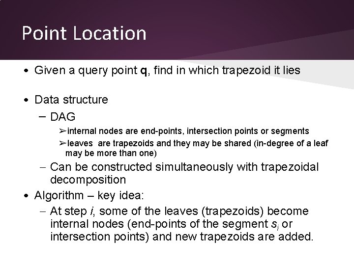
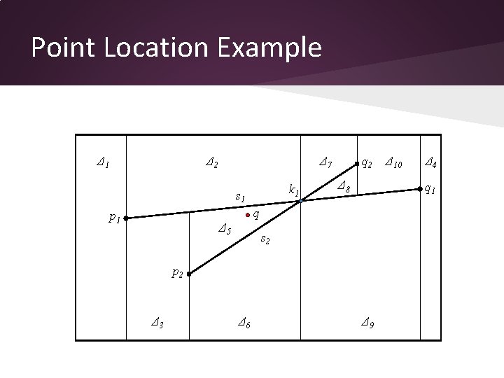
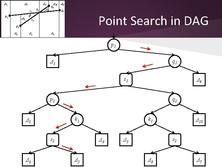
Point Location • Given a query point q, find in which trapezoid it lies • Data structure – DAG ➢internal nodes are end-points, intersection points or segments ➢leaves are trapezoids and they may be shared (in-degree of a leaf may be more than one) – Can be constructed simultaneously with trapezoidal decomposition • Algorithm – key idea: – At step i, some of the leaves (trapezoids) become internal nodes (end-points of the segment si or intersection points) and new trapezoids are added.

Point Location Example Δ 1 Δ 2 Δ 7 k 1 s 1 q 2 Δ 8 Δ 5 s 2 p 2 Δ 3 Δ 6 Δ 4 q 1 q p 1 Δ 10 Δ 9

Δ 1 Δ 2 Δ 7 s 1 p 1 Δ 5 k 1 Δ 8 Δ 10 q 2 Δ 4 q 1 Point Search in DAG q s 2 p 2 Δ 3 Δ 6 Δ 9 p 1 q 1 Δ 1 s 1 Δ 4 p 2 q 2 k 1 Δ 3 s 2 Δ 6 k 1 Δ 9 Δ 5 Δ 10 s 2 Δ 3 Δ 8 Δ 7

Complexity Analysis Assumption: points (end of segment) are in “general position” = no two points lies in a same vertical line. = all x-coordinate are different. Later we will see how to lift this assumption.

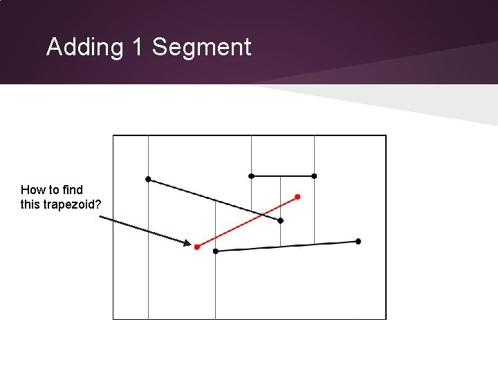
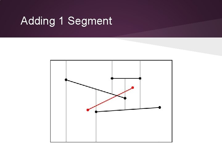
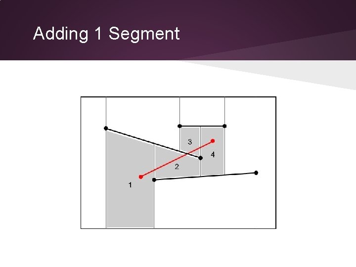
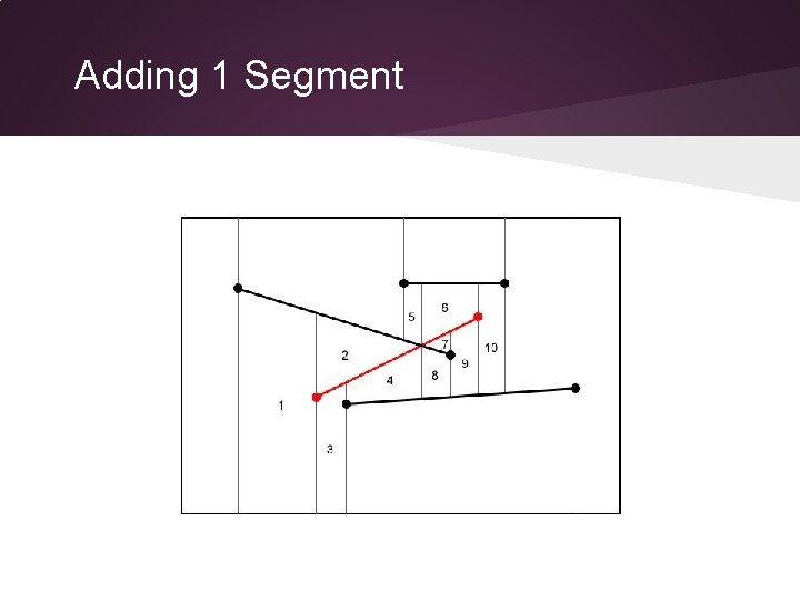
Complexity Analysis What is the complexity of adding one segment s? • find the left end point of segment s. • trace (and update) all trapezoids intersected by s.

Adding 1 Segment

Adding 1 Segment How to find this trapezoid?

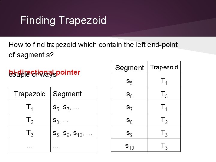
Finding Trapezoid How to find trapezoid which contain the left end-point of segment s? bi-directional couple of wayspointer Trapezoid Segment Trapezoid s 5 T 1 s 6 T 3 T 1 s 5, s 7, . . . s 7 T 1 T 2 s 8, . . . s 8 T 2 T 3 s 6, s 9, s 10, . . . s 9 T 3 . . . s 10 T 3

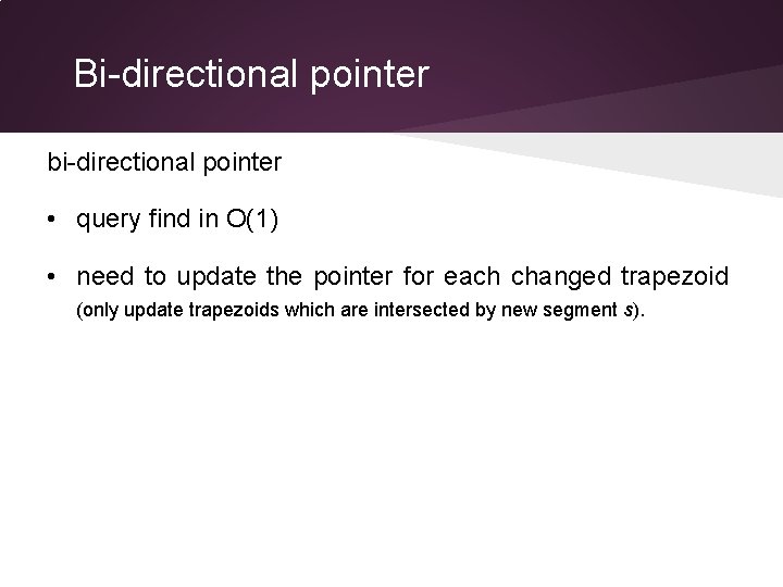
Bi-directional pointer bi-directional pointer • query find in O(1) • need to update the pointer for each changed trapezoid (only update trapezoids which are intersected by new segment s).

Adding 1 Segment

Adding 1 Segment

Adding 1 Segment

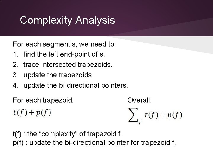
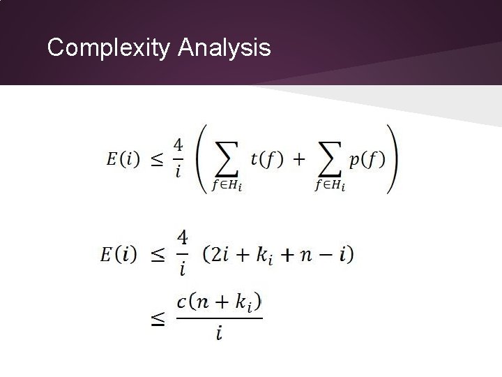
Complexity Analysis For each segment s, we need to: 1. find the left end-point of s. 2. trace intersected trapezoids. 3. update the trapezoids. 4. update the bi-directional pointers. For each trapezoid: Overall: t(f) : the “complexity” of trapezoid f. p(f) : update the bi-directional pointer for trapezoid f.

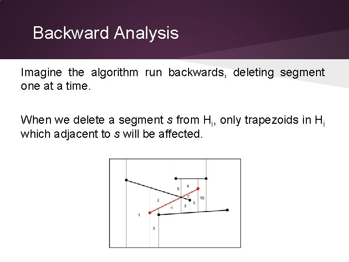
Backward Analysis Imagine the algorithm run backwards, deleting segment one at a time. When we delete a segment s from Hi, only trapezoids in Hi which adjacent to s will be affected.

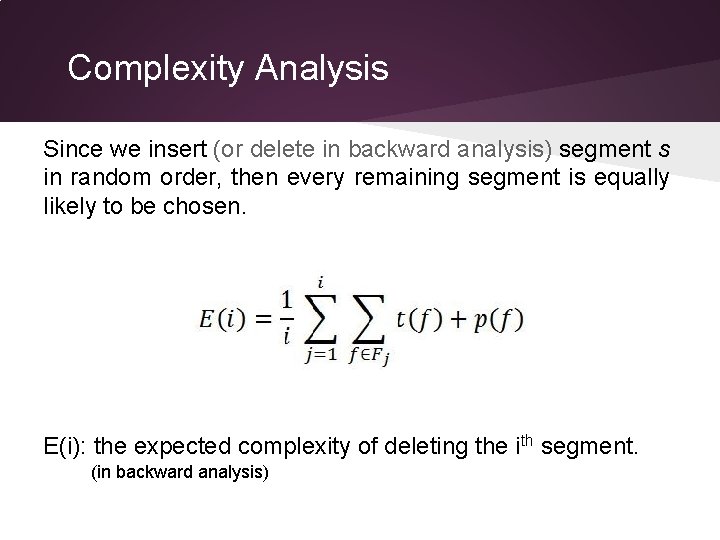
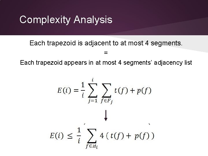
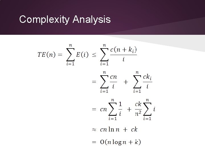
Complexity Analysis Since we insert (or delete in backward analysis) segment s in random order, then every remaining segment is equally likely to be chosen. E(i): the expected complexity of deleting the ith segment. (in backward analysis)

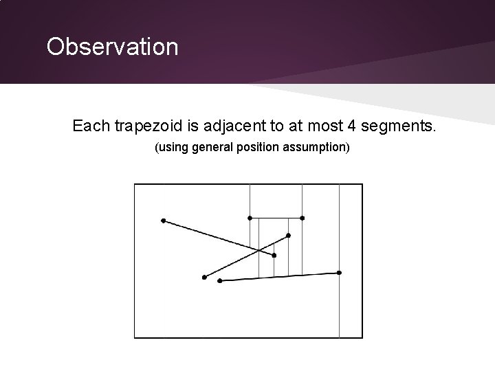
Observation Each trapezoid is adjacent to at most 4 segments. (using general position assumption)

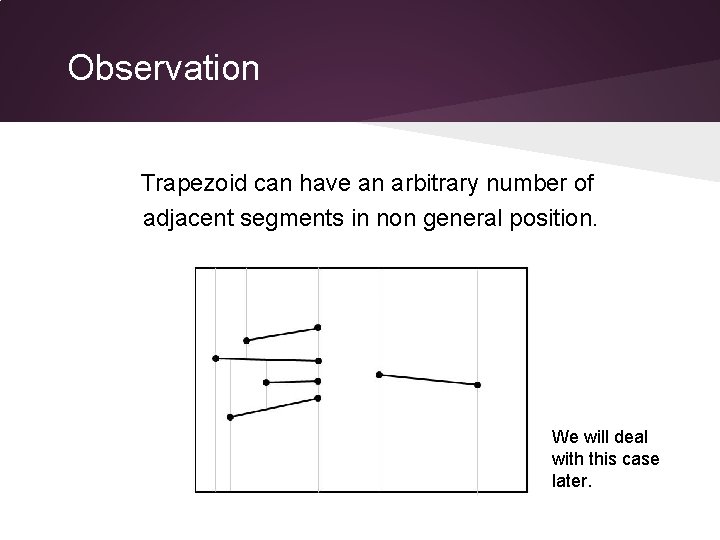
Observation Trapezoid can have an arbitrary number of adjacent segments in non general position. We will deal with this case later.

Complexity Analysis Each trapezoid is adjacent to at most 4 segments. = Each trapezoid appears in at most 4 segments’ adjacency list

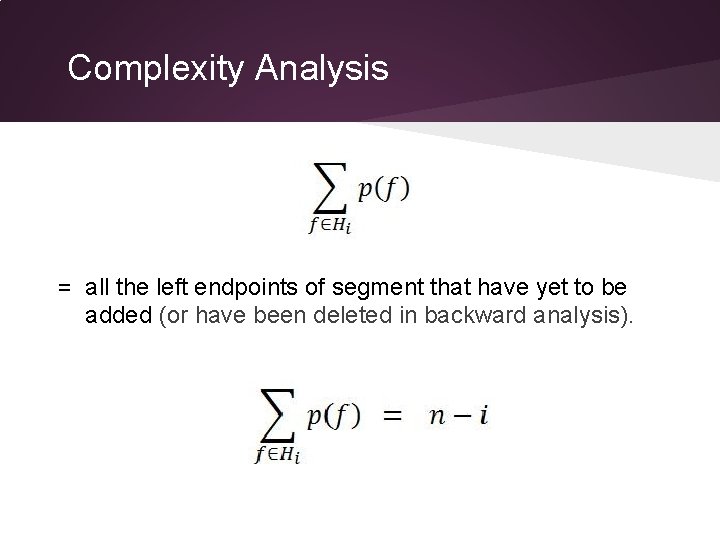
Complexity Analysis = all the left endpoints of segment that have yet to be added (or have been deleted in backward analysis).

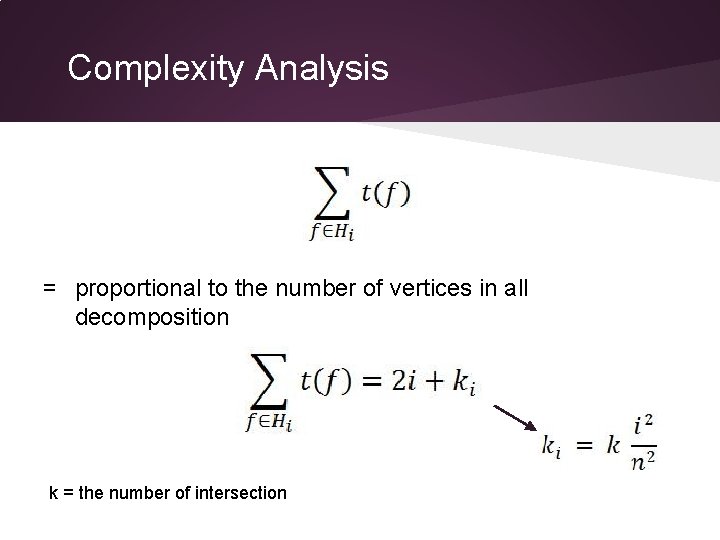
Complexity Analysis = proportional to the number of vertices in all decomposition k = the number of intersection

Complexity Analysis

Complexity Analysis

Randomized vs. Deterministic

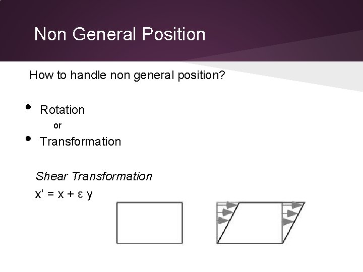
Non General Position How to handle non general position? • • Rotation or Transformation Shear Transformation x’ = x + ε y

Summary Voronoi Diagrams -- Use Fortune Algorithm Delaunay Triangulation -- Randomized Incremental Construction – Dual of Voronoi Trapezoidal Decomposition -- Randomized Incremental Construction

Conclusion • Widely used in various other areas. • We use it sometimes without even realising it. • Lot of potential of further development. • Numerous interesting open problems. http: //compgeom. cs. uiuc. edu/~jeffe/open/

Thank You

References Voronoi • Derek Johns, "An Optimal Algorithm for Computing 2 D Voronoi Diagrams Fortune's Sweep Algorithm", • • Available at http: //cgm. cs. mcgill. ca/~mcleish/644/Projects/Derek. Johns/Sweep. htm [Accessed February 2014] Dheeraj Kumar Singh, "Lecture 20: Voronoi Diagrams and Fortunes Algorithm", Available at http: //intinno. iitkgp. ernet. in/courses/91/wfiles/37906 [Accessed February 2014] Voronoi Diagrams, Available at http: //ima. udg. edu/~sellares/Com. Geo/Vor 2 D_1. ppt [Accessed February 2014] Delaunay Triangulation • http: //www. cs. umd. edu/~mount/754/Lects/754 lects. pdf • http: //www. cs. uu. nl/geobook/interpolation. pdf • http: //www. comp. nus. edu. sg/~hcheng/academic/courses/cs 5237/notes/04. pdf • http: //www. comp. nus. edu. sg/~hcheng/academic/courses/cs 5237/notes/05. pdf • http: //www. comp. nus. edu. sg/~tantc/ioi_training/CG/l 9 cs 4235. pdf • http: //www. comp. nus. edu. sg/~tantc/ioi_training/CG/l 10 cs 4235. pdf • http: //groups. csail. mit. edu/graphics/classes/6. 838/F 01/lectures/Delaunay 2 D. ppt Trapezoidal Decomposition • • Rajeev Motwani, Prabhakar Raghavan, “Randomized Algorithms”, 1995 Subhash Suri, “Point Location”, Available at http: //www. cs. ucsb. edu/~suri/cs 235/Location. pdf