Geomathematical and geostatistical characters of some clastic Neogene

Geomathematical and geostatistical characters of some clastic Neogene hydrocarbon reservoirs in the Croatia (“Stochastic simulations and geostatistics”, J. Geiger) Tomislav Malvić Szeged, December 2011

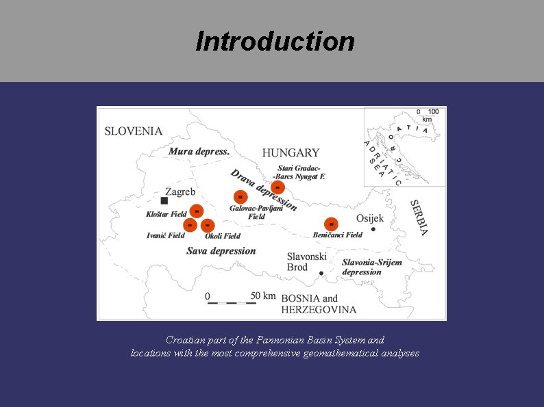
Introduction Croatian part of the Pannonian Basin System and locations with the most comprehensive geomathematical analyses

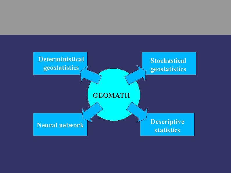
Deterministical geostatistics Stochastical geostatistics GEOMATH Neural network Descriptive statistics

➲ Such analyses had been done in the largest Croatian depressions: Sava and Drava. ➲ The most of them were geostatistical, but also some of them included neural networks and advanced statistics. ➲ Geostatistical analyses had been based on 10 -25 data points. ➲ Neural and statistical analyses was performed on several dozens data points.

➲ The Sava Depression: ➲ The Drava Depression: ➲ Kloštar, ➲ Stari Gradac-Barcs Nyugat, ➲ Ivanić, ➲ Molve, ➲ Okoli Fields. ➲ Beničanci, ➲ Galovac-Pavljani, ➲ The Bjelovar Subdepression with set of vertical variograms.

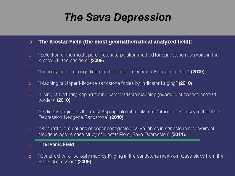
The Sava Depression ➲ The Kloštar Field (the most geomathematical analyzed field): ➲ “Selection of the most appropriate interpolation method for sandstone reservoirs in the Kloštar oil and gas field” (2008); ➲ “Linearity and Lagrange linear multiplicator in Ordinary Kriging equation” (2009); ➲ “Mapping of Upper Miocene sandstone facies by Indicator Kriging” (2010); ➲ “Using of Ordinary Kriging for indicator variable mapping (example of sandstone/marl border)” (2010); ➲ “Ordinary Kriging as the most Appropriate Interpolation Method for Porosity in the Sava Depression Neogene Sandstone” (2010); ➲ “Stochastic simulations of dependent geological variables in sandstone reservoirs of Neogene age: A case study of Kloštar Field, Sava Depression” (2011). ➲ The Ivanić Field: ➲ “Construction of porosity map by Kriging in the sandstone reservoir, Case study from the Sava Depression” (2008).

The Drava Depression ➲ The Beničanci Field: ➲ “Application of methods: Inverse distance weighting, ordinary kriging and collocated cokriging in porosity evaluation, and comparison of results on the Beničanci and Stari Gradac fields in Croatia” (2003); ➲ “Benefits of application of neural network in porosity estimation (example the Beničanci Field)” (2007); ➲ “Significance of the amplitude attribute in porosity prediction, Drava Depression Case Study” (2008); ➲ “Cokriging geostatistical mapping and importance of quality of seismic attribute(s)” (2009). ➲ The Molve Field: ➲ “Relation between Effective Thickness, Gas Production and Porosity in Heterogeneous Reservoir: and Example from the Molve Field, Croatian Pannonian Basin” (2010). ➲ The Galovac-Pavljani Field: ➲ “Application of deterministic and stochastic methods in OOIP calculation: Case study of Galovac-Pavljani field” (2007).

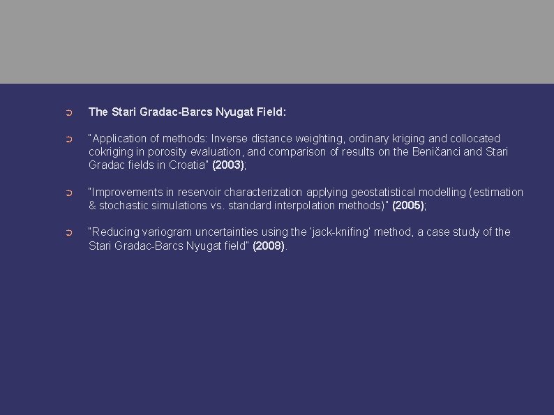
➲ The Stari Gradac-Barcs Nyugat Field: ➲ “Application of methods: Inverse distance weighting, ordinary kriging and collocated cokriging in porosity evaluation, and comparison of results on the Beničanci and Stari Gradac fields in Croatia” (2003); ➲ “Improvements in reservoir characterization applying geostatistical modelling (estimation & stochastic simulations vs. standard interpolation methods)” (2005); ➲ “Reducing variogram uncertainties using the ‘jack-knifing’ method, a case study of the Stari Gradac-Barcs Nyugat field” (2008).

The 1 st period 1999 -2006 “Begining” Recognizing of possible geomathematical applications in the analyses of HC reservoirs in the Croatian part of the Pannonian Basin System.

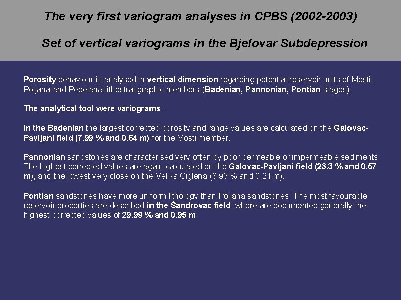
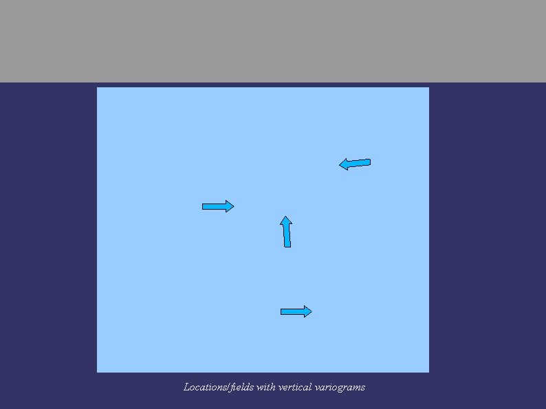
The very first variogram analyses in CPBS (2002 -2003) Set of vertical variograms in the Bjelovar Subdepression Porosity behaviour is analysed in vertical dimension regarding potential reservoir units of Mosti, Poljana and Pepelana lithostratigraphic members (Badenian, Pannonian, Pontian stages). The analytical tool were variograms. In the Badenian the largest corrected porosity and range values are calculated on the Galovac. Pavljani field (7. 99 % and 0. 64 m) for the Mosti member. Pannonian sandstones are characterised very often by poor permeable or impermeable sediments. The highest corrected values are again calculated on the Galovac-Pavljani field (23. 3 % and 0. 57 m), and the lowest very close on the Velika Ciglena (8. 95 % and 0. 21 m). Pontian sandstones have more uniform lithology than Poljana sandstones. The most favourable reservoir properties are described in the Šandrovac field, where are documented generally the highest corrected values of 29. 99 % and 0. 95 m.

Locations/fields with vertical variograms

Variogram ranges in Badenian clastics

Variogram ranges in Lower Pontian clastics (Poljana Sandstones)

Variogram ranges in Lower Pontian clastics (Poljana Sandstones)

The very first variogram analyses in CPBS (2003) Different interpolator algorithms Results have been compared of the porosity evaluation for: -Inverse Distance Weighting, -Ordinary Kriging and -Collocated Cokriging. The comparison had been made in the: -Beničanci field, -Stari Gradac-Barcs Nyugat field. The accuracy is determined by: -the geological evaluation of the isoporosity line shapes and -calculation of the mean square error (MSE). The best solution was acquired by the Collocated Cokriging method.

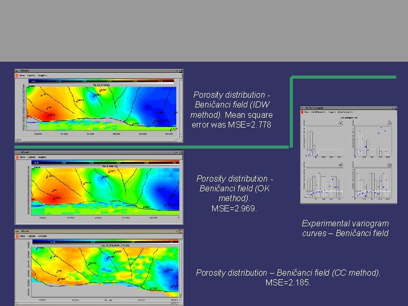
Porosity distribution Beničanci field (IDW method). Mean square error was MSE=2. 778 Porosity distribution Beničanci field (OK method). MSE=2. 969. Experimental variogram curves – Beničanci field Porosity distribution – Beničanci field (CC method). MSE=2. 185.

The 2 nd period 2007 -2010 “Mature geomathematical explorations” Numerous methods had been applied in the most of the large HC reservoirs in the CPBS

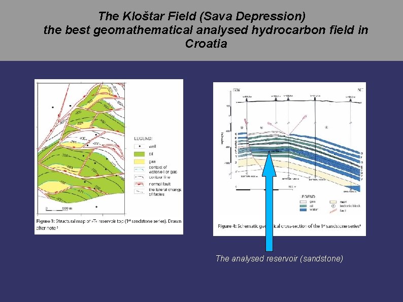
The Kloštar Field (Sava Depression) the best geomathematical analysed hydrocarbon field in Croatia The analysed reservoir (sandstone)

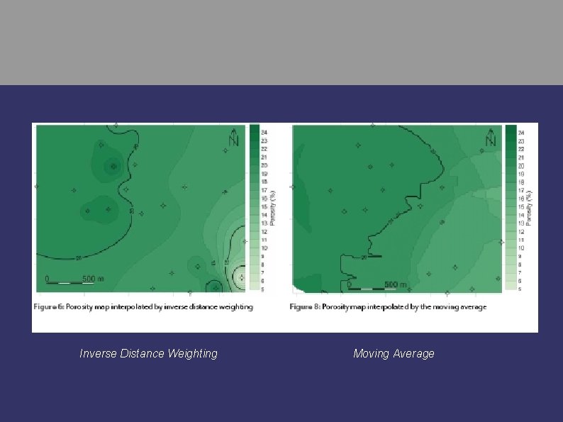
Inverse Distance Weighting Moving Average

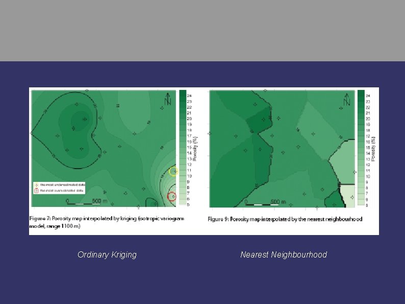
Ordinary Kriging Nearest Neighbourhood

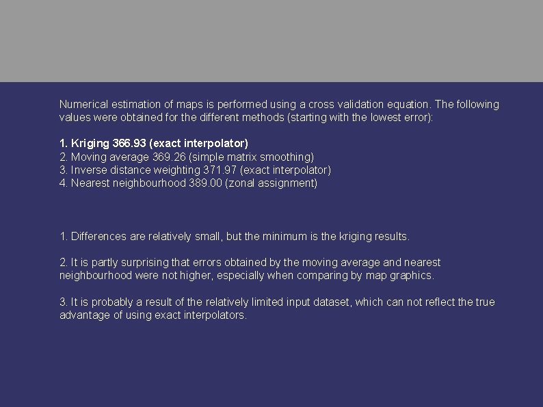
Numerical estimation of maps is performed using a cross validation equation. The following values were obtained for the different methods (starting with the lowest error): 1. Kriging 366. 93 (exact interpolator) 2. Moving average 369. 26 (simple matrix smoothing) 3. Inverse distance weighting 371. 97 (exact interpolator) 4. Nearest neighbourhood 389. 00 (zonal assignment) 1. Differences are relatively small, but the minimum is the kriging results. 2. It is partly surprising that errors obtained by the moving average and nearest neighbourhood were not higher, especially when comparing by map graphics. 3. It is probably a result of the relatively limited input dataset, which can not reflect the true advantage of using exact interpolators.

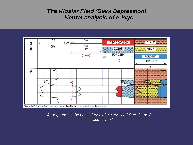
The Kloštar Field (Sava Depression) Neural analysis of e-logs Well log representing the interval of the 1 st sandstone “series” saturated with oil

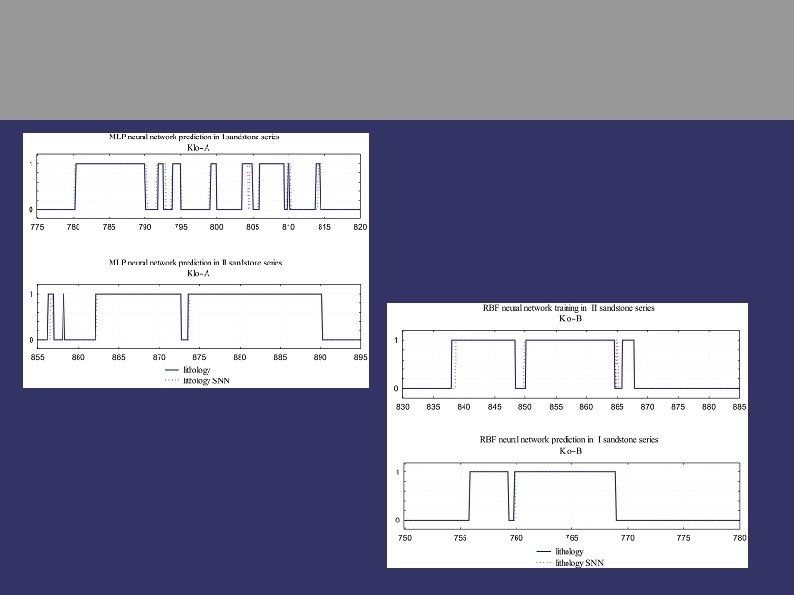
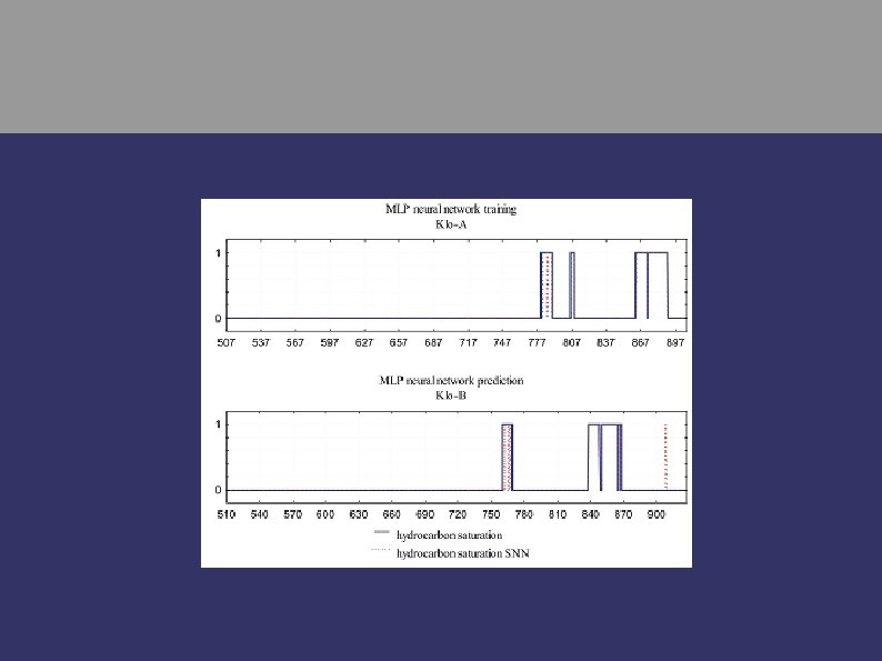
When determining the lithological component in wells Klo–A and Klo–B with RBF and MLP neural networks, achieved is excellent correspondence between true and predicted values. Prediction of hydrocarbon saturation in well Klo–B with a neural network trained in well Klo–A gave excellent correspondence between true and predicted values. Results show the great potential of neural networks’ application in petroleum geology research, where they could be used to quickly acquire results from well logs, to obtain vertical and lateral correlation of such logs, and to solve other petroleum geology problems.

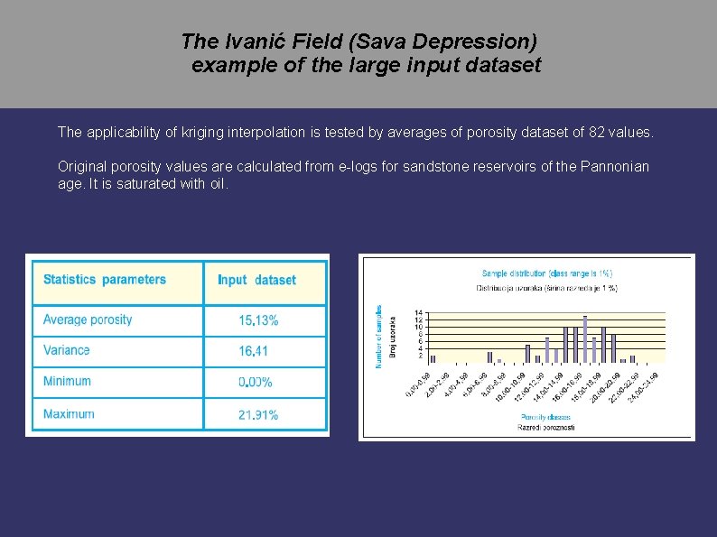
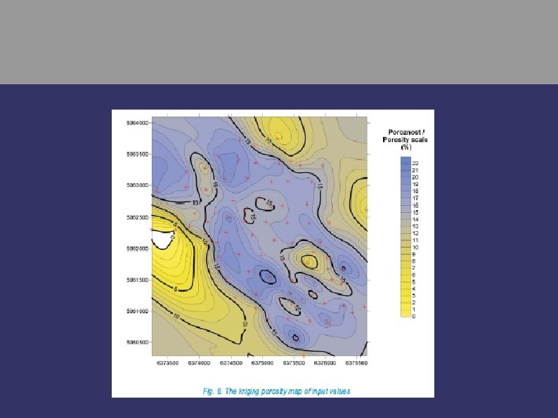
The Ivanić Field (Sava Depression) example of the large input dataset The applicability of kriging interpolation is tested by averages of porosity dataset of 82 values. Original porosity values are calculated from e-logs for sandstone reservoirs of the Pannonian age. It is saturated with oil.

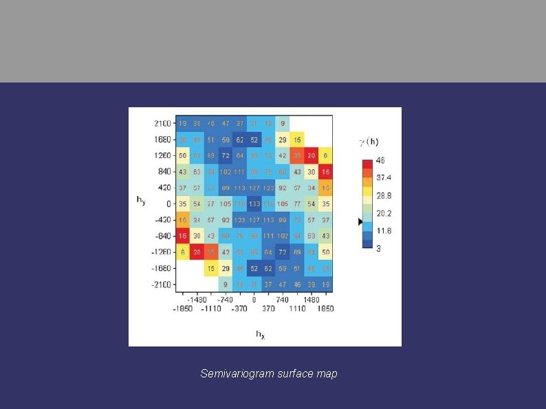
Semivariogram surface map

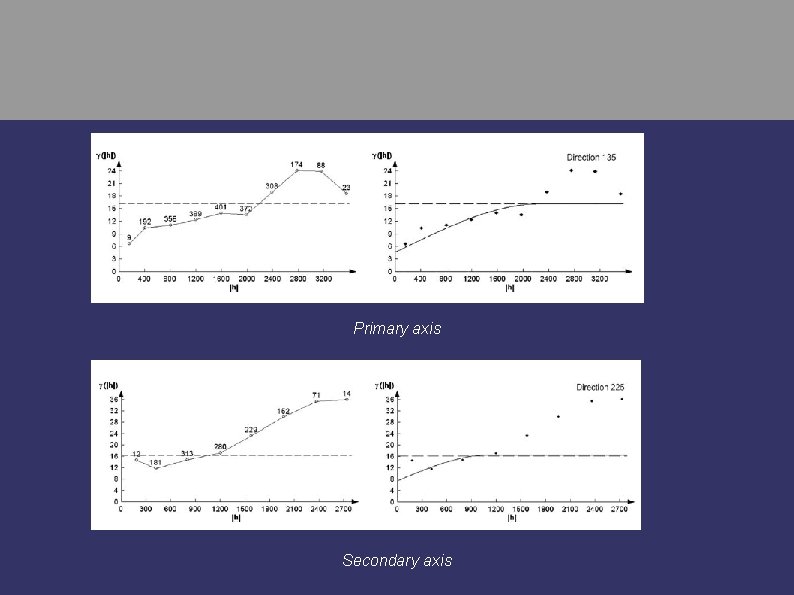
Primary axis Secondary axis

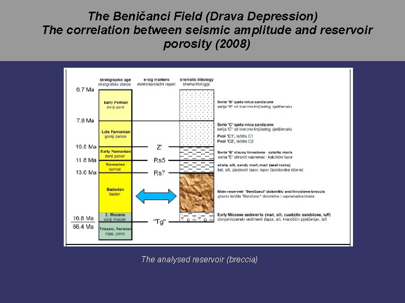
The Beničanci Field (Drava Depression) The correlation between seismic amplitude and reservoir porosity (2008) The analysed reservoir (breccia)

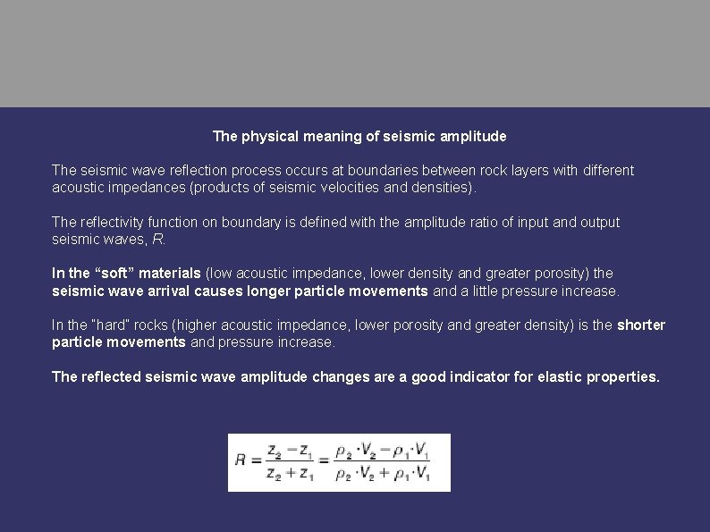
The physical meaning of seismic amplitude The seismic wave reflection process occurs at boundaries between rock layers with different acoustic impedances (products of seismic velocities and densities). The reflectivity function on boundary is defined with the amplitude ratio of input and output seismic waves, R. In the “soft” materials (low acoustic impedance, lower density and greater porosity) the seismic wave arrival causes longer particle movements and a little pressure increase. In the “hard” rocks (higher acoustic impedance, lower porosity and greater density) is the shorter particle movements and pressure increase. The reflected seismic wave amplitude changes are a good indicator for elastic properties.

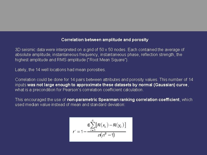
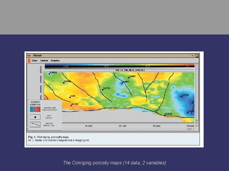
Correlation between amplitude and porosity 3 D seismic data were interpreted on a grid of 50 x 50 nodes. Each contained the average of absolute amplitude, instantaneous frequency, instantaneous phase, reflection strength, the highest amplitude and RMS amplitude (“Root Mean Square”). Lately, the 14 well locations had mean porosities. Correlation could be done for 14 pairs between attributes and porosity values. This number of 14 inputs was not large enough to approximate these datasets by normal (Gaussian) curve, what is a precondition for Pearson’s correlation coefficient calculation. This encouraged the use of non-parametric Spearman ranking correlation coefficient, which used median value instead of mean and standard deviation:

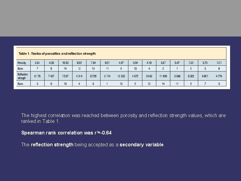
The highest correlation was reached between porosity and reflection strength values, which are ranked in Table 1. Spearman rank correlation was r’=-0. 64 The reflection strength being accepted as a secondary variable.

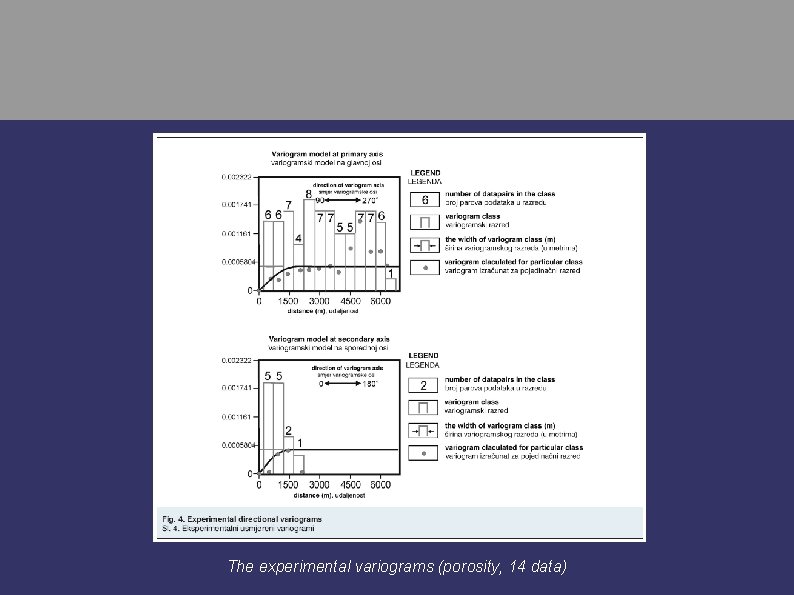
The experimental variograms (porosity, 14 data)

The Cokriging porosity maps (14 data, 2 variables)

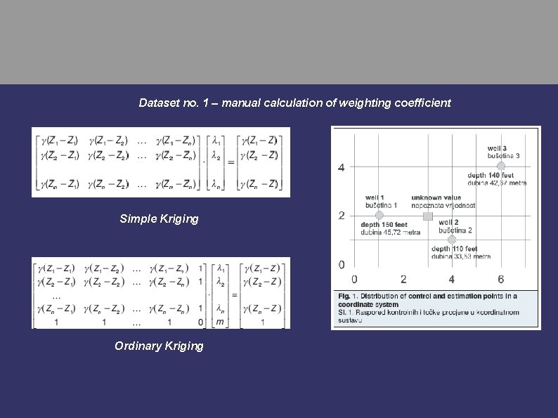
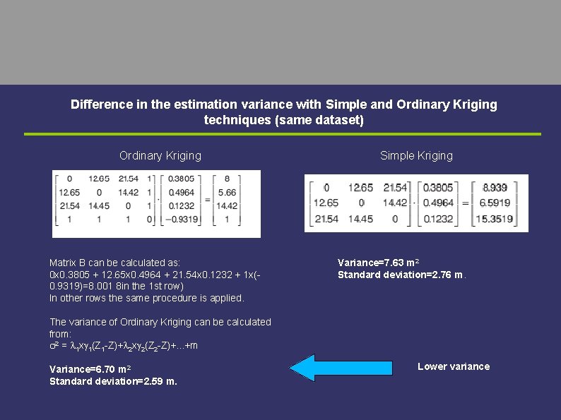
Theoretical work on Ordinary Kriging equations (2009) Linearity and Lagrange Linear Multiplicator in the Equations of Ordinary Kriging The equations of Simple and Ordinary Kriging are compared to outline their differences in the estimation procedure. Emphasis is given to the Lagrange multiplicator as a variable that allows the minimization of variance in Ordinary Kriging. A detailed presentation of equation sets provides a better understanding of the Simple and Ordinary Kriging algorithms for geological engineers, as the two most-used geostatistical techniques (included Indicator Kriging as the third). The conclusion includes proposals for the determination of the Lagrange multiplicator value in any Ordinary Kriging equation.

Dataset no. 1 – manual calculation of weighting coefficient Simple Kriging Ordinary Kriging

Difference in the estimation variance with Simple and Ordinary Kriging techniques (same dataset) Ordinary Kriging Matrix B can be calculated as: 0 x 0. 3805 + 12. 65 x 0. 4964 + 21. 54 x 0. 1232 + 1 x(0. 9319)=8. 001 8 in the 1 st row) In other rows the same procedure is applied. Simple Kriging Variance=7. 63 m 2 Standard deviation=2. 76 m. The variance of Ordinary Kriging can be calculated from: 2 = 1 x 1(Z 1 -Z)+ 2 x 2(Z 2 -Z)+. . . +m Variance=6. 70 m 2 Standard deviation=2. 59 m. Lower variance

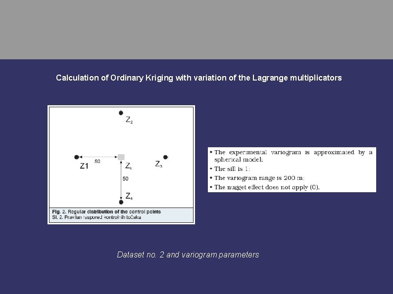
Calculation of Ordinary Kriging with variation of the Lagrange multiplicators Dataset no. 2 and variogram parameters

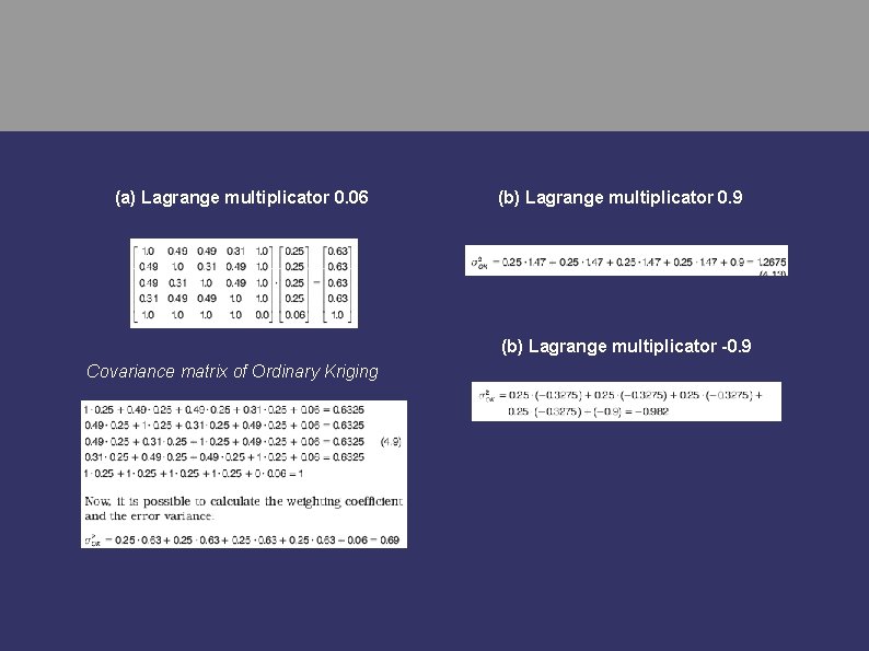
(a) Lagrange multiplicator 0. 06 (b) Lagrange multiplicator 0. 9 (b) Lagrange multiplicator -0. 9 Covariance matrix of Ordinary Kriging

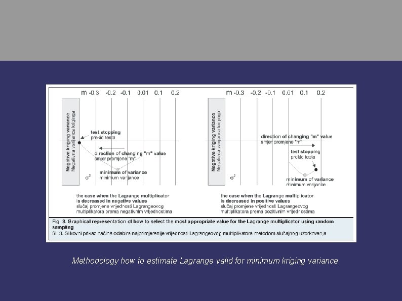
Methodology how to estimate Lagrange valid for minimum kriging variance

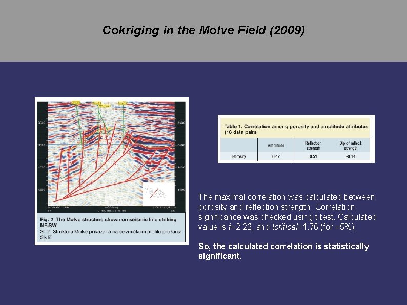
Cokriging in the Molve Field (2009) The maximal correlation was calculated between porosity and reflection strength. Correlation significance was checked using t-test. Calculated value is t=2. 22, and tcritical=1. 76 (for =5%). So, the calculated correlation is statistically significant.

The secondary variable is sampled at much more grid nodes than primary (2 500 vs. 16 nodes). It is why anisotropic experimental variogram is modelled from secondary variable data. This model is defined by: - Azimuth of primary axis 120º; - Lag-spacing about 350 m; - Primary range 4 000 m (spherical theoretical model without nugget); - Secondary range 2 900 m (spherical theoretical model without nugget).

The 3 rd period 2010 -2011 “Advanced and specific applications” Application of Indicator Kriging and using of simulation as regular tool

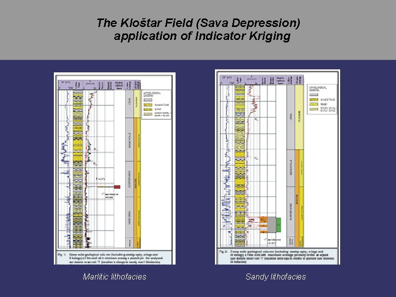
The Kloštar Field (Sava Depression) application of Indicator Kriging Marlitic lithofacies Sandy lithofacies

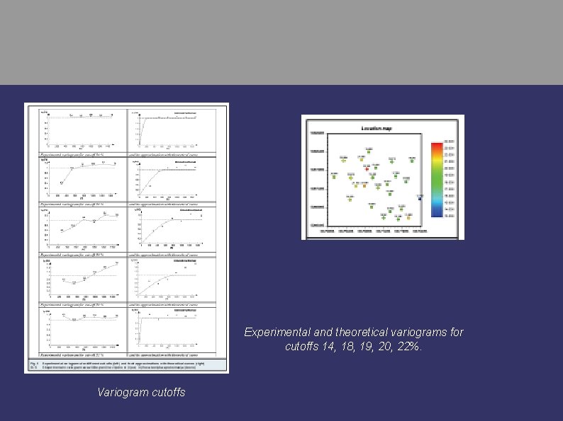
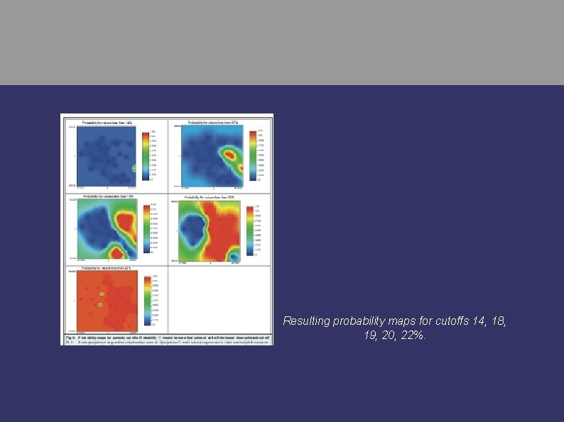
Experimental and theoretical variograms for cutoffs 14, 18, 19, 20, 22%. Variogram cutoffs

Resulting probability maps for cutoffs 14, 18, 19, 20, 22%.

1. Most of the kriging techniques are linear, but some of them are not. In fact, these are linear techniques applied on some non-linear transformation of the data. 2. Indicator transformation presented in analysis is one of such non-linear transformation and Indicator Kriging is non-linear technique as well. 3. Such application in this analysis resulted in indicator variograms for different porosity cutoffs and in set of probability maps for such cutoffs. 4. Using of these maps revealed the areal extension of porosity probability below defined cutoff.

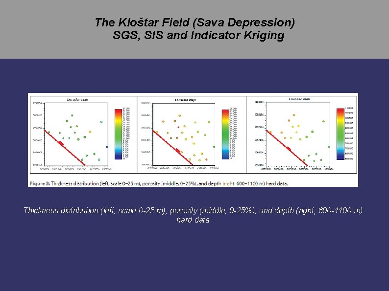
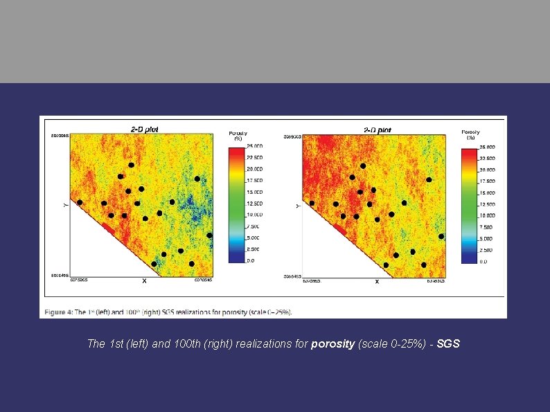
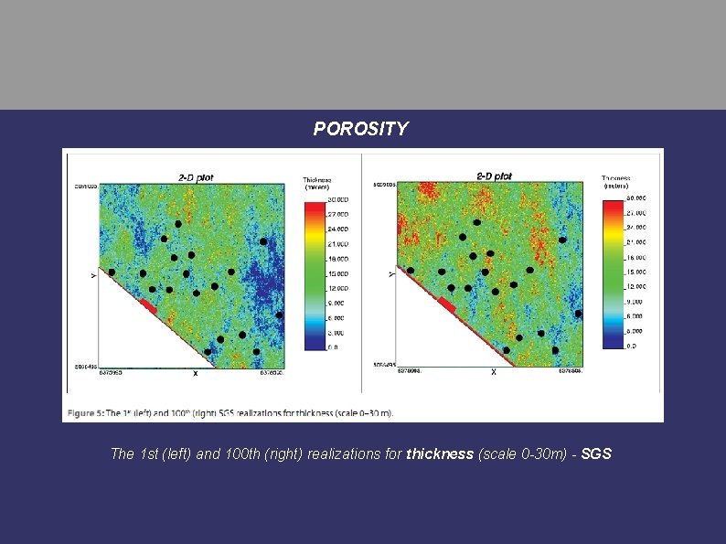
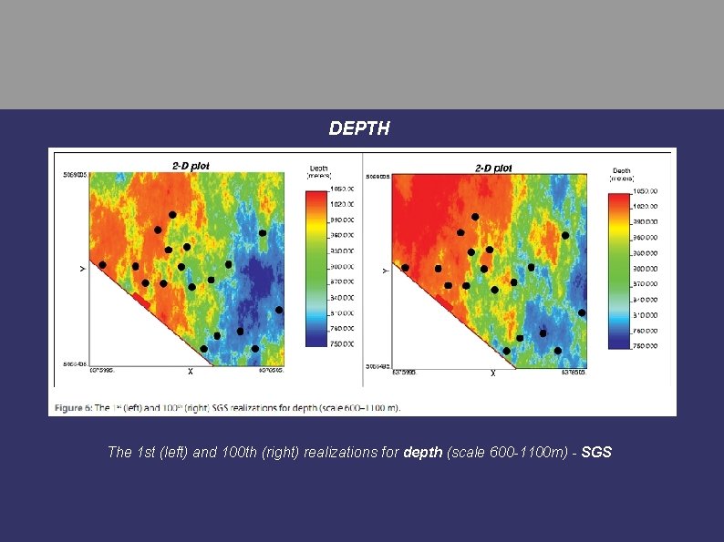
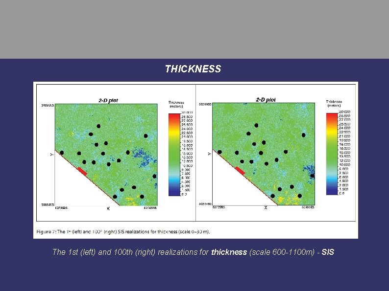
The Kloštar Field (Sava Depression) SGS, SIS and Indicator Kriging Thickness distribution (left, scale 0 -25 m), porosity (middle, 0 -25%), and depth (right, 600 -1100 m) hard data

In deterministic solution (that is also “zero” realization for simulation) the following values are always known: a) Mean value, variance (µ, σ2); b) Kriging variance (σ2); c) The interval allowed for simulated values (determined from the relationship between the mean and the variance); d) If the allowed interval encompasses three standard deviations (± 3σ) around a mean (µ) each cell, then 99% of all possible solutions are included. When all previous values are known and the type of simulation is defined, then the values of all model “blank” cells can be estimated using the SGS method.

The 1 st (left) and 100 th (right) realizations for porosity (scale 0 -25%) - SGS

POROSITY The 1 st (left) and 100 th (right) realizations for thickness (scale 0 -30 m) - SGS

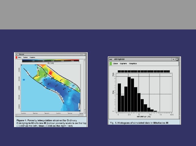
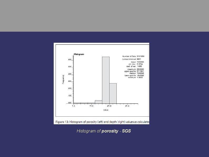
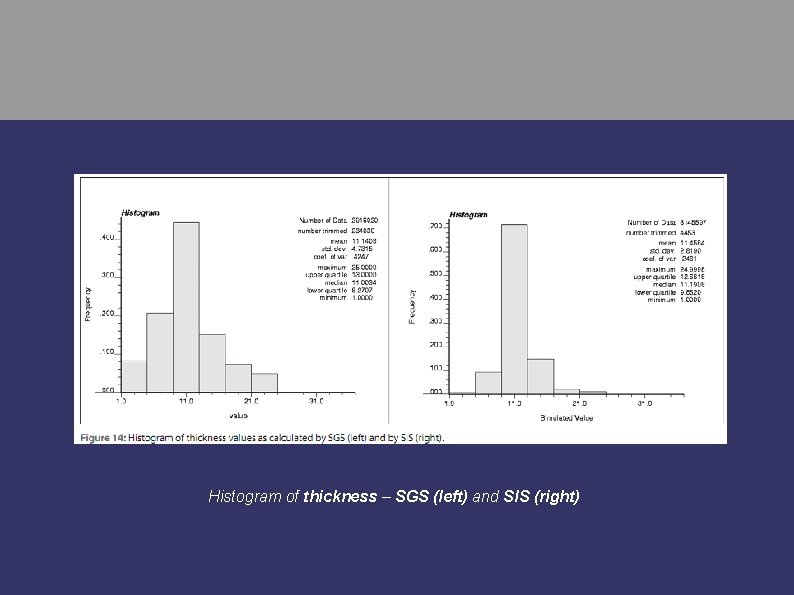
Histogram of porosity - SGS

DEPTH The 1 st (left) and 100 th (right) realizations for depth (scale 600 -1100 m) - SGS

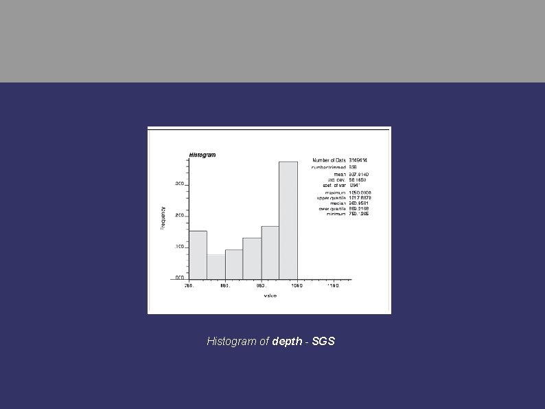
Histogram of depth - SGS

THICKNESS The 1 st (left) and 100 th (right) realizations for thickness (scale 600 -1100 m) - SIS

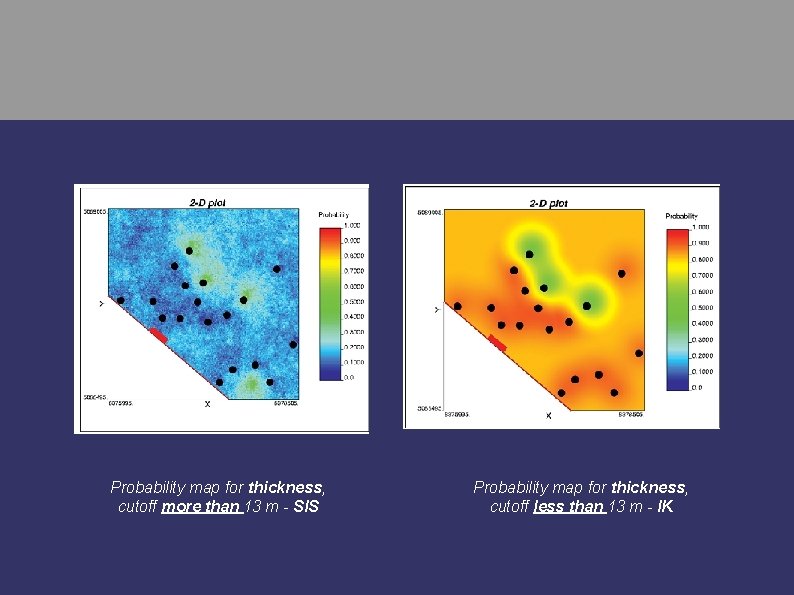
Probability map for thickness, cutoff more than 13 m - SIS Probability map for thickness, cutoff less than 13 m - IK

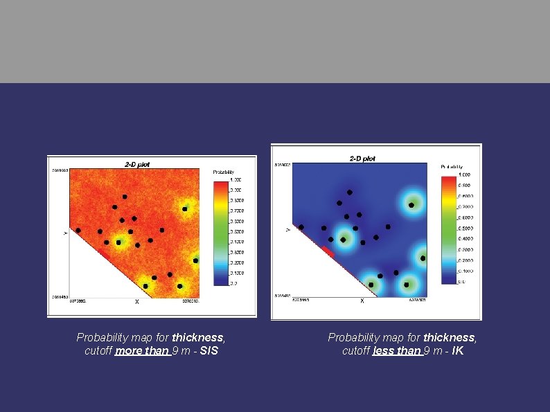
Probability map for thickness, cutoff more than 9 m - SIS Probability map for thickness, cutoff less than 9 m - IK

Histogram of thickness – SGS (left) and SIS (right)

Conclusions Practical development of geostatistics can be done in several ways. In presented examples it can be easily followed through simple three phases: 1. The simple and comprehensive application of variogram analysis (modelling); 2. The first using of different, usual (linear) kriging techniques (Simple and Ordinary Kriging); 3. The next “jump” on “non-linear” Indicator Kriging; 4. Theoretical analysis of kriging equations – i. e. the “basic” techniques Simple and Ordinary K. ; 5. The using of simulation, mostly the simplest – Sequential Gaussian Simulations; 6. Combination of Indicator Kriging and (Sequential) Indicator Simulations and mutual interpretation; 7. Using of simulation for obtaining new (hopefully) more descriptive histograms.

Selection of geological variable: 1. Theoretically it can be any reservoir variable; 2. Preferable is selection of variable with (theoretically) normal distribution (like porosity) or lognormal (permeability, but rarely). Regarding other part of geomathematics: 1. The “clasicall” descriptive statistics or t-test or F-test can be useful in introductory analysis of raw data and reveal some distribution characteristics or data group connections; 2. The application of neural networks is different tool that can be connected with geostatistics only occasionally or locally, e. g. , in some mapping application with several algorithms or Neural Kriging; 3. The neural algorithms are proven good tool for vertical analysis of e-logs.