Geology 56706670 Inverse Theory 8 Apr 2019 Last

Geology 5670/6670 Inverse Theory 8 Apr 2019 Last time: Optimal Interpolation • Optimal interpolation (or “kriging”, after Danie Krige) uses geostatistics of samples of a regionalized variable to calculate the best estimate and uncertainty of the variable at an unsampled location • For this, uses the variogram, or expected value of differences as a function of distance between measurements ( ): (related to autocovariance as: • The optimal estimate is given by in which the weights wi on measurements xi are solved via the system of equations: • And the estimation variance is then: © A. R. Lowry 2019

Example: Interpolation of PACES database gravity measurements to a grid: • Semivariance at mean distance 200 m is already 1. 5 m. Gal; 1 km = 3. 6 m. Gal, 2 km = 5. 2 m. Gal (!!!) • Obviously some areas (valley bottoms, populated, lotsa roads) pretty densely measured; some untouched…

Uncertainty mostly over 5 m. Gal, up to 20 in wilderness areas. Gravity here is draped over the gravity gradient… Note that some sites are evident outlier points! Poor network adjustment? Inconsistencies in elevation measurement/terrain correction?

Tikhonov Regularization: The generalized application of Tikhonov regularization is to solve linear problems of the form: by minimizing: for some appropriate choice of Tikhonov matrix, G, that serves as a low-pass filter operation on the model parameter space. This may be a difference operator, scaled identity matrix, or low-pass Fourier operator: 1 st derivative difference Scaled identity matrix

There are several plausible reasons for doing this: • If the physics kernel (G matrix) is ill-conditioned (which is often the case: note that least-squares inversion can be a high-pass filter operation!), this stabilizes the inversion • The minimization of the (weighted) model length term, , results in a smoothed solution that is aesthetically pleasing if the parameters sought are expected to be a continuous field in time or space BUT: • This means that Tikhonov regularization is completely analogous (if not equivalent) to damped least squares (choose l = q!), Singular Value Decomposition, Levenberg & Levenberg-Marquardt damping (for nonlinear problems!), and stochastic or Bayesian inversion…

The differences come down to how empirical versus rigorous is the choice of regularization damping. Arguably, the most rigorous approach would be to impose a stochastic or Bayesian inversion using the covariance matrix of the parameters being sought (presuming that the covariance properties are known!)

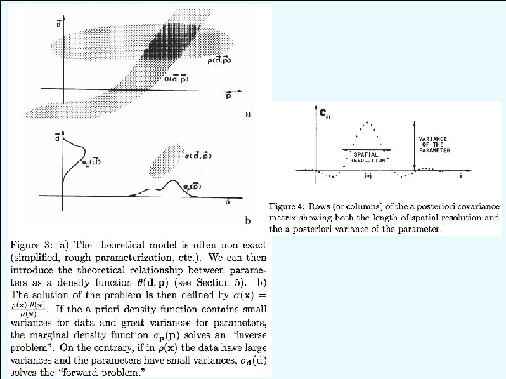
Tarantola & Valette 1982: Inverse Problems = Quest for Information Goals: • Represent both data and model parameters as probability density functions • Allow for non-exact physics (due to discretization or incomplete theory) by also representing physical relationships as probability density functions General goals of inverse theory: • Valid for linear & nonlinear problems • Valid for overdetermined & underdetermined problems • Consistent given a transformation of variables • Allow for generalized error (non-Gaussian, asymmetric) • Allow for generalized (e. g. </>; smooth) constraints/ assumptions • General enough to incorporate errors in theory

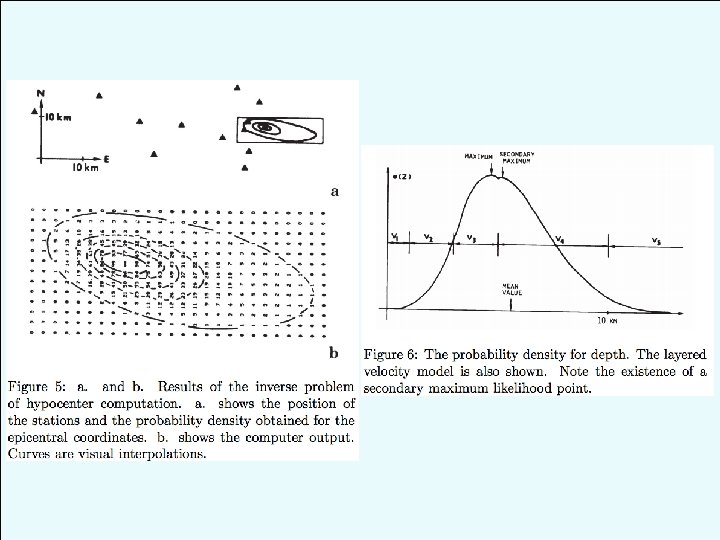
Tarantola & Valette 1982

An example inverse approach: Joint inversion of seismic reflection/gravity/MT data for subsalt imaging de Stefano et al. , Geophysics, 76(3) 2011 • Use a Bayesian objective function for minimization • “Simultaneous Joint Inversion” (SJI) solves for shared, unshared parameters and their relationships (e. g. v. P/ )

Single domain Cross-section Linked v = 2 km/s; 2. 07 g/cm 3 v = 6 v=5 2. 60 2. 72 Plan-view (1250 m) Synthetic velocity model Single domain inversions Linked (assumed Gardner’s law)

Initial model Linked (crossgradients) Single domain SJI

SJI MT