Geographic Information Systems GIS SGO 1910 SGO 4930

Geographic Information Systems (GIS) SGO 1910 & SGO 4930 Fall 2005

Revised Schedule n Week 43 (October 25) Geographic Databases Chapters 10 n Week 44 (Nov. 1) Geographic Analysis Chapters 14, 15 Week 45 (Nov. 8) Mid-term Quiz II Map Production Chapter 12 GIS and Society Chapter 18 n n Week 46 (Nov. 15) n Week 47 (November 22) NO CLASS n Week 48 Final Exam Dec 1

Oslo Project n The aim of this project is to integrate what you have learned in GIS lectures and labs through practical experience. Working in groups of three or four, you will address a spatial issue in Oslo (e. g. resource distribution, inequality) through the collection, mapping and analysis of data, which will then be presented in a concise professional report that is no more than 12 pages long, including maps and references.

Groups You may select your own group, or we can create groups for you. Groups should be established this week in lab – please email me the members of your group. n Graduate students have the option of doing an independent project related to their own research, or the Oslo project in a group. n

New Textbook? ? GIS - Geographic Information Systems for the Social Sciences: Investigating Space and Place (Steinbergy, S. J. and Steinberg, S. L. 2005. Sage Publications) n Replace Longley et al. ? Supplement it? n

Geographic Databases

A GIS can answer the question: What is where? n WHAT: Characteristics of attributes or features. n WHERE: In geographic space.

A GIS links attribute and spatial data n Attribute Data n n Flat File Relations n Map Data n n Point File Line File Area File Topology

Flat File Database Attribute Record Value Value Record Value

13 11 2 12 10 7 POLYGON “A” 5 4 9 2 8 1 6 3 1 1 xy 2 xy 3 xy 4 xy 5 xy 6 xy 7 xy 8 xy 9 xy 10 x y 11 x y 12 x y 13 x y Points File Arc/node map data structure with files File of Arcs by Polygon A: 1, 2, Area, Attributes 1 1, 2, 3, 4, 5, 6, 7 2 1, 8, 9, 10, 11, 12, 13, 7 Arcs File Figure 3. 4 Arc/Node Map Data Structure with Files.

What is a Data Model? A logical construct for the storage and retrieval of information. n Attribute data models are needed for the DBMS. n The origin of DBMS data models is in computer science. n

Definitions Database – an integrated set of data on a particular subject n Geographic (=spatial) database - database containing geographic data of a particular subject for a particular area n Database Management System (DBMS) – software to create, maintain and access databases n

A DBMS contains: Data definition language n Data dictionary n Data-entry module n Data update module n Report generator n Query language n

Advantages of Databases n n n Avoids redundancy and duplication Reduces data maintenance costs Applications are separated from the data n n Applications persist over time Support multiple concurrent applications Better data sharing Security and standards can be defined and enforced

Disadvantages of Databases Expense n Complexity n Performance – especially complex data types n Integration with other systems can be difficult n

Characteristics of DBMS (1) n Data model support for multiple data types n e. g MS Access supports Text, Memo, Number, Date/Time, Currency, Auto. Number, Yes/No, OLE Object, Hyperlink, Lookup Wizard Load data from files, databases and other applications n Index for rapid retrieval n

Characteristics of DBMS (2) Query language – SQL n Security – controlled access to data n n Multi-level groups Controlled update using a transaction manager n Backup and recovery n

Role of DBMS System Task Geographic Information System • • • Data load Editing Visualization Mapping Analysis Database Management System • • Storage Indexing Security Query Data

Retrieval n n The ability of the DBMS or GIS to get back on demand data that were previously stored. Geographic search is the secret to GIS data retrieval. Many forms of data organization are incapable of geographic search. GIS systems have embedded DBMSs, or link to a commercial DBMS.

Types of DBMS Model Hierarchical n Network n Relational - RDBMS n Object-oriented - OODBMS n Object-relational - ORDBMS n

Historically, databases were structured hierarchically in files. . . Norge Oppland Bærum Akershus Asker Hordaland Ski

Relational DBMS Data stored as tuples (tup-el), conceptualized as tables n Table – data about a class of objects n Two-dimensional list (array) n Rows = objects n Columns = object states (properties, attributes) n Tuple? ? ? A row in a relational table; synonymous with record, observation. A set of elements.

Relation Rules Only one value in each cell (intersection of row and column) n All values in a column are about the same subject n Each row is unique n No significance in column sequence n No significance in row sequence n

Table Column = property Row = object Table = Object Classes with Geometry called Feature Classes

Relational Join n Fundamental query operation Table joins use common keys (column values) Table (attribute) join concept has been extended to geographic case

Relational Data Bases Patient Record Key Check-in 42 2/1/96 78 2/3/96 Purchase Record Item Date Skate Board 2/1/96 Baseball Bat 2/1/96 Accident Report Date Injury 2/1/96 Broken Leg 2/2/96 Concussion 2/2/96 Cut on Ear Price 49. 95 17. 99 Name John Smith Sylvia Jones Robert Doe File Check Out Room No. 2/4/96 N 763 2/4/96 N 712 Customer John Smith James Brown Key 42 654 123 File Key 42 978 File Location 75 Elm Street 12 State Street 2323 Broad Street

Most DBMS are now relational databases. n Based on multiple flat files for records, with dissimilar attribute structures, connected by a common key attribute.

Retrieval Operations Searches by attribute: find and browse. n Data reorganization: select, renumber, and sort. n Compute allows the creation of new attributes based on calculated values. n

Spatial Retrieval Operations n n Attribute queries are not very useful for geographic search. In a map database the records are features. The spatial equivalent of a find is locate, the GIS highlights the result. Spatial equivalents of the DBMS queries result in locating sets of features or building new GIS layers.

The Retrieval User Interface n n n GIS query is usually by command line, batch, or macro. Most GIS packages use the GUI of the computer’s operating system to support both a menu-type query interface and a macro or programming language. SQL is a standard interface to relational databases and is supported by many GISs.

SQL n n Structured (Standard) Query Language – (pronounced SEQUEL) Developed by IBM in 1970 s Now de facto and de jure standard for accessing relational databases Three types of usage n n n Stand alone queries High level programming Embedded in other applications

Types of SQL Statements n Data Definition Language (DDL) n n n Data Manipulation Language (DML) n n n Create, alter and delete data CREATE TABLE, CREATE INDEX Retrieve and manipulate data SELECT, UPDATE, DELETE, INSERT Data Control Languages (DCL) n n Control security of data GRANT, CREATE USER, DROP USER

Spatial Relations n n n n n Equals – same geometries Disjoint – geometries share common point Intersects – geometries intersect Touches – geometries intersect at common boundary Crosses – geometries overlap Within– geometry within Contains – geometry completely contains Overlaps – geometries of same dimension overlap Relate – intersection between interior, boundary or exterior

Spatial Methods n n n n Distance – shortest distance Buffer – geometric buffer Convex. Hull – smallest convex polygon geometry Intersection – points common to two geometries Union – all points in geometries Difference – points different between two geometries Sym. Difference – points in either, but not both of input geometries

Spatial Search Buffering is a spatial retrieval around points, lines, or areas based on distance. n Overlay is a spatial retrieval operation that is equivalent to an attribute join. n

Identify

Recode OR

Data overlay

Overlay

Types of overlay operations And n Or n Max n Min n

Buffer (raster) +1

Buffer (vector)

Complex Retrieval: Map Algebra n Combinations of spatial and attribute queries can build some complex and powerful GIS operations, such as weighting.

Summary Database – an integrated set of data on a particular subject n Databases offer many advantages over files n Relational databases dominate n

Part II: Working with Attributes in Arc. GIS

Issues to discuss how attribute data is stored in a table of rows and columns n how attribute data is associated with features n tabular field types supported in Arc. GIS n types of table relationships n how tables can be related to each other n how to join tables based on a common field n

Review n A geographic database contains both spatial and tabular data. The spatial data contains feature shape and location information, while the tabular data contains the attributes for the features. Often, feature attributes are contained in multiple tables.

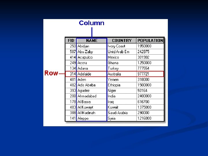
Anatomy of a Table n n Each table in a database has the same basic format: an array of rows and columns. Rows are also called records, and columns are also called fields. Some tables, like a feature class's default feature attribute table, have a preset number of columns. For instance, a polygon coverage's feature attribute table has four standard columns: Area, Perimeter, Coverage#, and Coverage-ID, while a line shapefile's feature attribute table has only one default column, named Shape. Other tables are completely userdefined.

n n The table has three user-added columns: Name, Country, and Population. Arc. Map automatically adds a third column (FID) for display purposes. The name of this column may be different depending on the type of data source. For example, it is called FID for a coverage or shapefile, OBJECTID for a geodatabase feature class, and Order_ID for a grid. Because some databases and some operations do not support fields with blanks in their names, you should avoid creating fields that contain them. In addition, every column in a table should have a unique name but columns in the same table can have a variety of formats. NOTE: Norwegian “æ å ø” can also create problems, as can decimal formats (10, 1 versus 10. 1).

Tabular data field types n n Tables are capable of storing date, number, and text values, but most tabular formats have several different field types to store this information. Choosing the best field type for the values to be stored is an important consideration. Also, the available field types can vary between tabular formats. In general, you can store numbers, text, and dates. Specifically supported formats in Arc. Catalog™ include short integer, long integer, float, double, text, date, object-id, and blob.

Information stored in tables is organized by fields and field types. When defining a table's fields, be aware that each database has its own rules defining what names and characters are permitted.

Arc. GIS Tabular Formats n n Arc. GIS supports the use of multiple formats for storing and managing tabular data. Each of Arc. GIS software's primary spatial formats has its own native format. Coverages use INFO -formatted tables; shapefiles store their attributes in d. BASE (. dbf) format; geodatabases rely on the format of their supporting RDBMS (Oracle, for example). Deciding on the proper format in which to store attribute information is an important part of database design and can affect the efficiency with which you are able to access feature attributes. To facilitate sharing data that's in different formats, Arc. Catalog and Arc. Toolbox contain tools to convert between the various tabular formats. In addition, some formats, such as the coverage, can link to independent tables regardless of their format.

Tabular information can be stored in a variety of formats. In this case, feature information is stored in the coverage feature attribute table, data about the owners is stored in d. BASE format, and tax information is stored in a relational database format.

Associating Tables n Because features often have many attributes, most database design guidelines promote organizing your database into multiple tables—each focused on a specific topic—instead of one large table containing all the necessary fields. This scheme is more efficient because it eliminates duplicate information in the database–you store the information only once in one table. Tables can be "connected" so that when you need information that isn't in the current table, you can access it from a table associated with it.

n Two tables can be connected if there is a similar field in each table containing common values. Each table must have at least one field containing unique values for each record; in database terminology, this field is called the primary key. Even if there are duplicate values in all the other fields, the primary key ensures that each row will be unique.

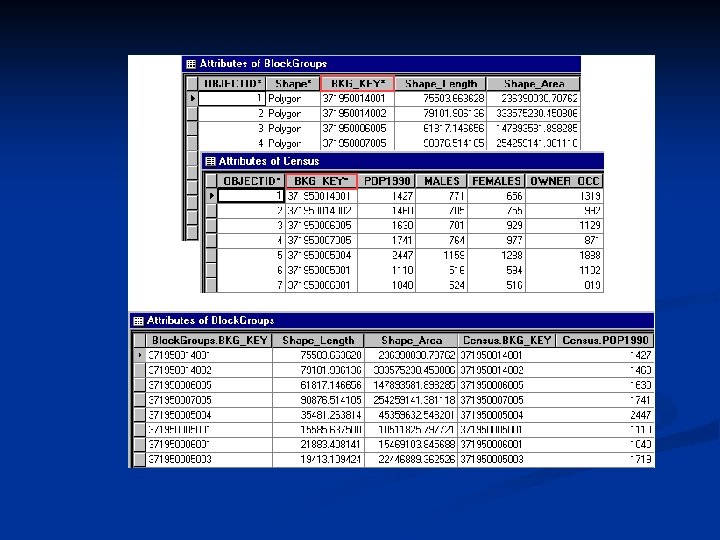
n Row uniqueness is important when connecting two tables because you want to make sure the correct rows are matched together. As a general rule, you connect tables from a primary key field in one table to the common field (called the foreign key) in the other table. In the next graphic, the ZONE_CODE field exists in both tables, contains common values in each, and has unique values in each row in the attribute table on the right. The tables can be connected based on this field.

In each table above, ZONE_CODE contains the same values—codes for zoning types. The attribute table on the right also contains the descriptions for each code; this information is not stored in the feature attribute table, but it is information that users will want to access often. The tables will be connected so that the zoning descriptions can be easily accessed.

Table Relationships n In Arc. Map, you can connect two tables using either a join or a relate. In order to know which method to use, you need to know how individual records in each table relate to one another. You need to know if one or more than one record in the first table is associated with one or more than one record in the second table. There are four possible relationship types (also called cardinality): one-to-one, one-to-many, many-to-one, and many-to-many.

Cardinality n n A property of a relationship between objects in a database, describing how many objects of type A are associated with how many objects of type B. Relationships can have one-to-one, one-to-many, many-to-one, and many-to-many cardinalities. For example, one parcel can have one owner (one-toone), one parcel can have many owners (one-tomany), many parcels can have one owner (many-toone), or many parcels can have many different owners (many-to-many).

Connecting tables with joins n n You can connect two tables together in Arc. Map using a join. Join works with shapefiles, coverages, and geodatabase feature classes. Once the tables are connected, you can query, symbolize, and analyze your data based on the joined values. Table joins are designed for one-to-one or many-toone relationships. For other cardinalities you should use a relate instead of a join. If you join two tables that have one-to-many or many-to-many cardinality, you will omit all records after the first match for each primary key value.

n n When joining two tables, the names of the common fields need not be identical but the fields must be the same type (e. g. , text, date, float, etc. ). The Arc. Map Join Data dialog is where you specify which tables you want to join and which fields contain the values that will match. Joined tables are not permanently connected. The fields from one table are appended to the other table. You can tell from which table a field originates because its source table name displays in its field name. You can remove a table join whenever you want. Table joins are “virtual”; that is, the two tables still exist as separate entities.

Connecting tables with relates n n Another way that you can connect tables in Arc. Map is by creating a relate. Like joining tables, relating tables defines a relationship between two tables and is also based upon a common field. Unlike joining tables, a relate doesn't append the fields of one table to the other. Instead, you access data in the related table by selecting records in one table and accessing the related records in the other table. You relate tables instead of joining them when there is a one-to-many or many-to-many relationship between the tables.

The Attributes of parcels table and the Owners table have a one-to-many relationship (a parcel may have more than one owner). The two tables are related based on the Parcel_no field. Selecting vacant parcels in the attribute table selects the records with matching parcel numbers in the related table.

n In Arc. Map, you create a relate in the Relate dialog by choosing the tables you want to relate and the fields in each that the relate will be based on. To access data in a related table, open one of the tables and select the records for which you want to display related records. Click Options, point to Related Tables, and click the name of the relate you want to access. The related table will display with the related records selected. It doesn’t matter which table you open, because in Arc. Map table relates are bi-directional.

n If your data is involved in both joins and relates, the order in which the joins and relates are created is significant. If you have a table for which you have created a relate and you join another table to it, the relate will be removed. If you perform a relate on a joined table, the relate is removed when the join is removed. As a general rule of thumb, it is best to create your joins, then add your relates.

Join n Suppose you have a parcels feature attribute table and another attribute table that contains the names of parcel owners. The graphic below shows a one-to-one relationship. Each parcel has only one owner, so each record in the feature attribute table will relate to one record in the owners attribute table. For this type of relationship, you would use a table join.

n The graphics below show both a one-to-many and a many-toone relationship. On the left, one parcel can have many owners; therefore, the relationship is one-to-many. On the right, many parcels can have one owner, resulting in a many-to -one relationship. For a one-to-many relationship, you should create a table relate; for a many-to-one relationship, you should create a table join.

n You can also have relationships where many features relate to many records in the other attribute table. In this situation, many parcels could have many owners. This is the most complex relationship and can be difficult to manage. For this type of relationship, you should associate the two tables using a table relate.

Other items to discuss sort, calculate, and freeze data in a table n create summary statistics n edit feature attributes using the Attributes dialog n use the Field Calculator to update attribute values n create a graph n create a report n

n There a number of ways you can display attribute data. You can change the way data is displayed in a table, and you can take data out of the table and display it as statistics or in a graph or report.

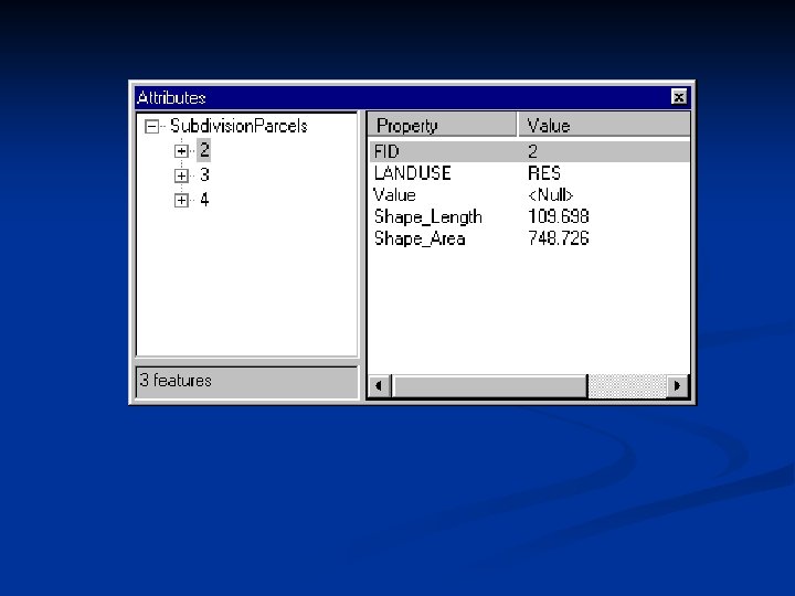
Access and edit attribute data in Arc. Map. n When you want to edit feature attributes, you start an editing session. When you're in an editing session, you can view the attributes of selected features by clicking the Attributes button to bring up the Attributes dialog. The Attributes dialog has two parts: a tree view on the left that lists each selected feature, and a pane on the right that shows the attribute values for the feature currently selected in the tree view.

n If you select features from more than one layer, each layer that contains selected features will be listed in the tree view. You can access individual selected features by expanding their layer

n If you select features from more than one layer, each layer that contains selected features will be listed in the tree view. You can access individual selected features by expanding their layer

n You can edit the attribute values for a single feature by clicking next to the field name and typing in the new value.

n If you want to change values for all the selected features at once, you can click the layer name and type the new value next to the field you want to update. In the graphic below, the OWNER values for all the selected homes are being changed to "Alvi Contracting. "

Table manipulation n You can manipulate tables to change how data is viewed. Right-clicking any field brings up a context menu with many choices. You can sort the record values in a selected field either in ascending or descending order. You can sort both numeric and character fields.

n You can calculate the values of selected records using the Field Calculator. In the Field Calculator, you can update all the values or a selected set of values in a field at one time.

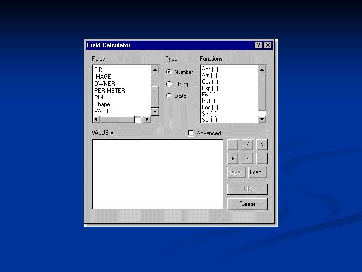
Using the Field Calculator n n In Arc. Map, you can edit feature attributes by creating simple calculations or logical expressions in the Field Calculator. The Field Calculator works on selected features or on all features in a layer if there are none selected. To access the Field Calculator, first start an editing session, then open the desired layer's attribute table by right-clicking the layer name in the Table of Contents. Choose Open Attribute Table and when the table displays, right-click the field you want to update. Choose Calculate Values to display the Field Calculator.

n To create an expression in the Field Calculator, you combine fields, functions, and operators. As you click on fields and functions, they appear in the expression box. You can also type directly into the box. The expression below will update the VALUE field with the results of multiplying each feature's area by 1. 5.

Freeze or unfreeze a column n Freezing a column locks a column as the left-most column in the table view. You can then use the horizontal scroll bar to see the other columns in the table. When you scroll, the frozen column remains in place while all other columns move. A frozen column is easily identified because it has a thick black line separating it from the other columns in the table.

Calculating statistics n After selecting features on the map or selecting records in a table, you may want to calculate simple summary statistics for the data. (Cchoose the Statistics option from Arc. Map's Selection menu) n After you select the layer and field in the feature attribute table for which you want statistics calculated, a list of summary statistics, as well as a frequency distribution chart, display in the Selection Statistics window.

Graphs in Arc. GIS n Values for Arc. GIS graphs come directly from feature attribute tables. You can represent your data and analysis results using many styles of graphs, including both two- and threedimensional graphs. Some graphs are better than others at presenting certain kinds of information. You should carefully consider the information you want to present before choosing a graph style.

n Once you've created a graph, you can add it to a map in Arc. Map's Layout View. When placed on the layout, a graph becomes a graphic element that you can size and position as desired. Once you've placed a graph on a layout, however, it becomes static and changes to the graph's source table will not be reflected in the graph.

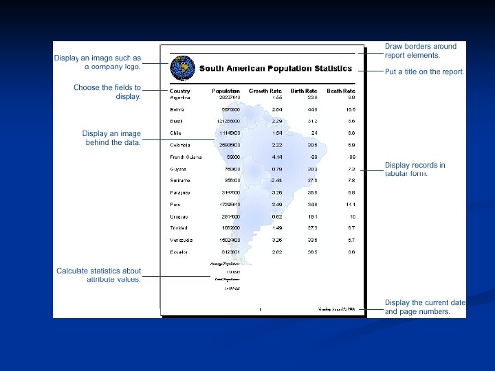
Reports n n A report presents tabular information about map features (from a feature attribute table) formatted in an attractive manner. You can choose which fields from your table you want to display and how you want to display them. Once you've created a report, you can place it on your map layout with your geographic data or save it as a file for distribution. A report includes a title, page numbers and the current date, summary statistics, images, borders, and, of course, the data from the feature attribute table.

n n Displaying your data in a report allows you to organize your data. You can sort records based on the values in one or more fields—given a list of cities, you could sort them by total population, for example. You can also group records and calculate summary statistics. For example, you could group cities by their country. It would then be easy to see which city has the largest population in a given country. You can also calculate summary statistics—sum, average, count, standard deviation, minimum, and maximum values. You can export reports to different file types, including Adobe's Portable Document Format (PDF), Rich Text Format (RTF), or plain text (TXT).