Geografiske informasjonssystemer GIS SGO 1910 SGO 4930 Vr

Geografiske informasjonssystemer (GIS) SGO 1910 & SGO 4930 Vår 2004 Foreleser: Karen O’Brien (karen. obrien@cicero. uio. no) Seminarleder: Gunnar Berglund (gunnarbe@student. sv. uio. no)

Outline v What is spatial analysis? v Queries and reasoning v Measurements

Spatial Analysis v Turns v by raw data into useful information adding greater informative content and value v Reveals patterns, trends, and anomalies that might otherwise be missed v Provides a check on human intuition v by helping in situations where the eye might deceive

Definitions v A method of analysis is spatial if the results depend on the locations of the objects being analyzed move the objects and the results change v results are not invariant (i. e. , they vary!) under relocation v v Spatial analysis requires both attributes and locations of objects v a GIS has been designed to store both

The Snow Map (cholera outbreaks in the 1850 s) Provides a classic example of the use of location to draw inferences v But the same pattern could arise from contagion (cholera spread through the air) v if the original carrier lived in the center of the outbreak v contagion was the hypothesis Snow was trying to refute today, a GIS could be used to show a sequence of maps as the outbreak developed v contagion would produce a concentric sequence, drinking water a random sequence v

Types of Spatial Analysis There are literally thousands of techniques v Six categories are used in this course, each having a distinct conceptual basis: v Queries and reasoning v Measurements v Transformations v Descriptive summaries v Optimization v Hypothesis testing v

Queries and Reasoning v. A GIS can respond to queries by presenting data in appropriate views v and allowing the user to interact with each view v It is often useful to be able to display two or more views at once v and to link them together v linking views is one important technique of exploratory spatial data analysis (ESDA)

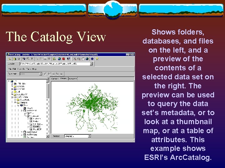
The Catalog View Shows folders, databases, and files on the left, and a preview of the contents of a selected data set on the right. The preview can be used to query the data set’s metadata, or to look at a thumbnail map, or at a table of attributes. This example shows ESRI’s Arc. Catalog.

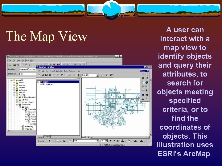
The Map View A user can interact with a map view to identify objects and query their attributes, to search for objects meeting specified criteria, or to find the coordinates of objects. This illustration uses ESRI’s Arc. Map.

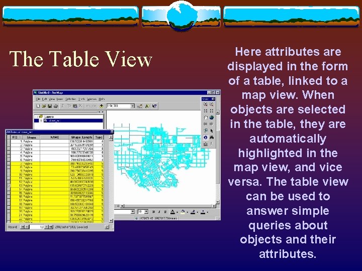
The Table View Here attributes are displayed in the form of a table, linked to a map view. When objects are selected in the table, they are automatically highlighted in the map view, and vice versa. The table view can be used to answer simple queries about objects and their attributes.

Measurements v Many tasks require measurement from maps v measurement of distance between two points v measurement of area, e. g. the area of a parcel of land v Such measurements are tedious and inaccurate if made by hand v measurement using GIS tools and digital databases is fast, reliable, and accurate

Measurement of Length v. A metric is a rule for determining distance from coordinates v The Pythagorean metric gives the straight-line distance between two points on a flat plane v The Great Circle metric gives the shortest distance between two points on a spherical globe v given their latitudes and longitudes

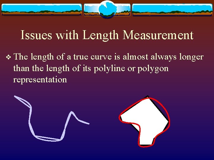
Issues with Length Measurement v The length of a true curve is almost always longer than the length of its polyline or polygon representation

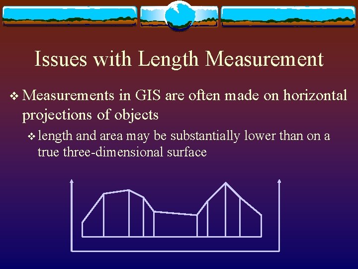
Issues with Length Measurement v Measurements in GIS are often made on horizontal projections of objects v length and area may be substantially lower than on a true three-dimensional surface

Measurement of Shape v Shape measures capture the degree of contortedness of areas, relative to the most compact circular shape v by comparing perimeter to the square root of area v normalized so that the shape of a circle is 1 v the more contorted the area, the higher the shape measure

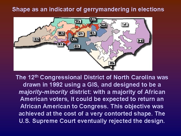
Shape as an indicator of gerrymandering in elections The 12 th Congressional District of North Carolina was drawn in 1992 using a GIS, and designed to be a majority-minority district: with a majority of African American voters, it could be expected to return an African American to Congress. This objective was achieved at the cost of a very contorted shape. The U. S. Supreme Court eventually rejected the design.

Slope and Aspect Calculated from a grid of elevations (a digital elevation model) v Slope and aspect are calculated at each point in the grid, by comparing the point’s elevation to that of its neighbors v usually its eight neighbors v but the exact method varies v in a scientific study, it is important to know exactly what method is used when calculating slope, and exactly how slope is defined v

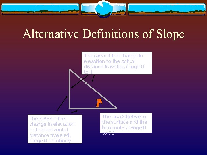
Alternative Definitions of Slope The ratio of the change in elevation to the actual distance traveled, range 0 to 1 The ratio of the change in elevation to the horizontal distance traveled, range 0 to infinity The angle between the surface and the horizontal, range 0 to 90

Transformations v Create new objects and attributes, based on simple rules v involving geometric construction or calculation v may also create new fields, from existing fields or from discrete objects

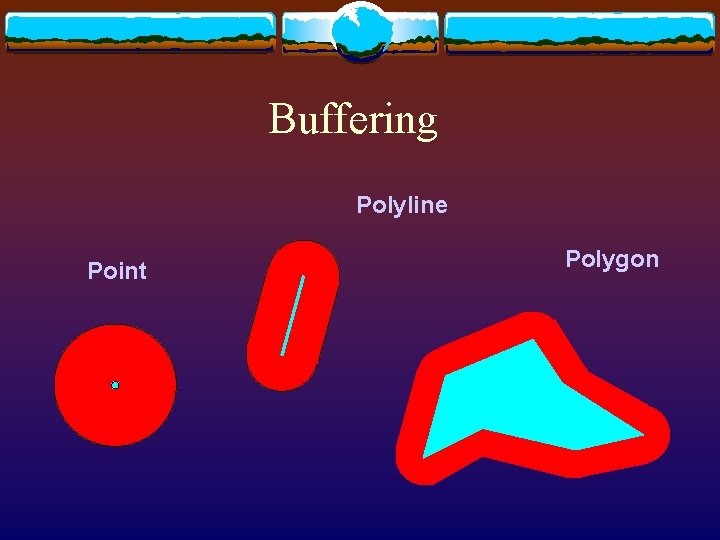
Buffering (Dilation) v Create a new object consisting of areas within a user-defined distance of an existing object v e. g. , to determine areas impacted by a proposed highway v e. g. , to determine the service area of a proposed hospital v Feasible in either raster or vector mode

Buffering Polyline Point Polygon

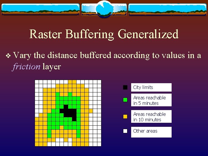
Raster Buffering Generalized v Vary the distance buffered according to values in a friction layer City limits Areas reachable in 5 minutes Areas reachable in 10 minutes Other areas

Point in Polygon Transformation v Determine whether a point lies inside or outside a polygon v generalization: assign many points to containing polygons v used to assign crimes to police precincts, voters to voting districts, accidents to reporting counties

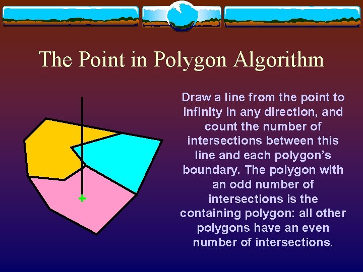
The Point in Polygon Algorithm Draw a line from the point to infinity in any direction, and count the number of intersections between this line and each polygon’s boundary. The polygon with an odd number of intersections is the containing polygon: all other polygons have an even number of intersections.

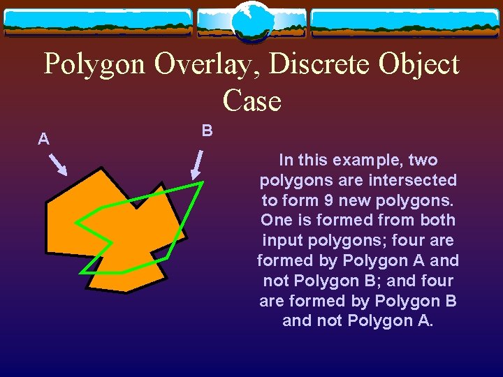
Polygon Overlay v Two case: for discrete objects and for fields v Discrete object case: find the polygons formed by the intersection of two polygons. There are many related questions, e. g. : v do two polygons intersect? v where areas in Polygon A but not in Polygon B?

Polygon Overlay, Discrete Object Case A B In this example, two polygons are intersected to form 9 new polygons. One is formed from both input polygons; four are formed by Polygon A and not Polygon B; and four are formed by Polygon B and not Polygon A.

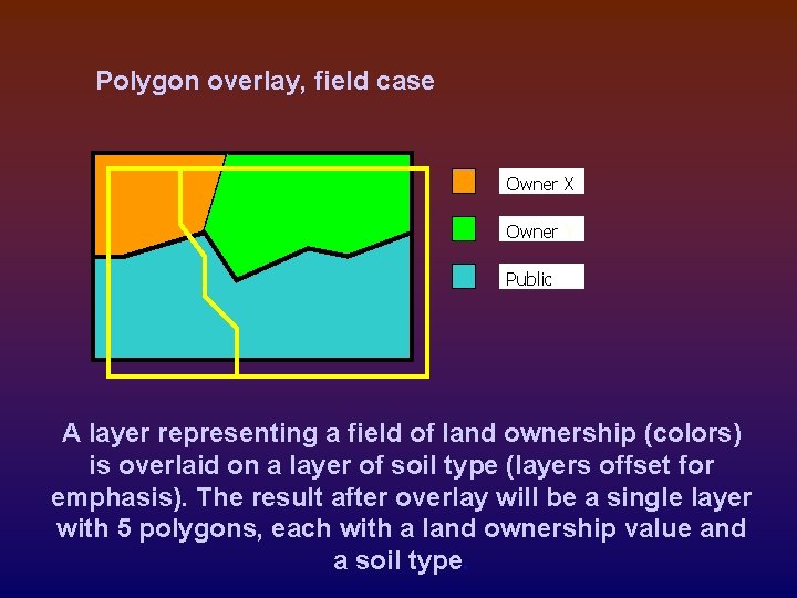
Polygon Overlay, Field Case v Two complete layers of polygons are input, representing two classifications of the same area v v e. g. , soil type and land ownership The layers are overlaid, and all intersections are computed creating a new layer each polygon in the new layer has both a soil type and a land ownership v the attributes are said to be concatenated v v The task is often performed in raster

Polygon overlay, field case Owner X Owner Y Public A layer representing a field of land ownership (colors) is overlaid on a layer of soil type (layers offset for emphasis). The result after overlay will be a single layer with 5 polygons, each with a land ownership value and a soil type.

Spurious or Sliver Polygons v In any two such layers there will almost certainly be boundaries that are common to both layers v e. g. following rivers The two versions of such boundaries will not be coincident v As a result large numbers of small sliver polygons will be created v these must somehow be removed v this is normally done using a user-defined tolerance v

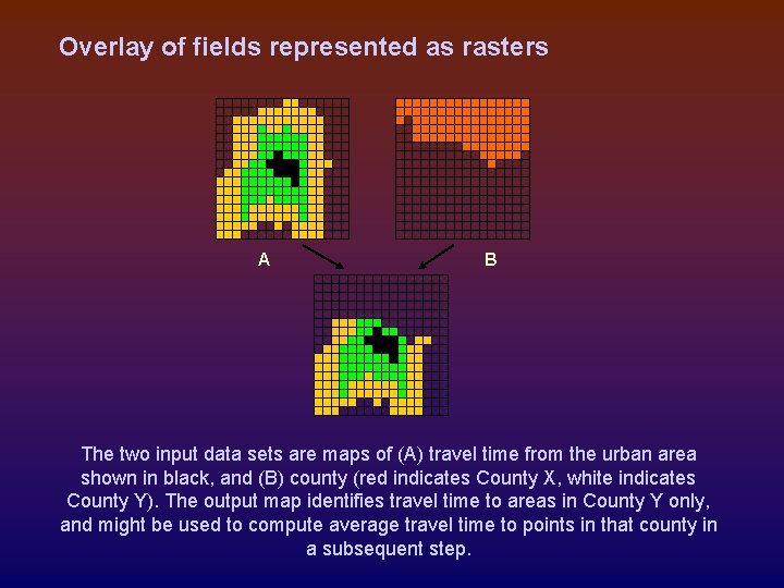
Overlay of fields represented as rasters A B The two input data sets are maps of (A) travel time from the urban area shown in black, and (B) county (red indicates County X, white indicates County Y). The output map identifies travel time to areas in County Y only, and might be used to compute average travel time to points in that county in a subsequent step.