Geoff Willis Risk Manager Geoff Willis Juergen Mimkes


 =B*(x-G)*(EXP(-P*(x-G))) It")
 =B*(x-G)*(EXP(-P*(x-G))) B =10*No*P*P So:")
 =10*No*P*P*(x-G)*(EXP(-P*(x-G))) Parameters varied: P")


 =10*No*(2/((Ko/No)-G))*(x-G)*(EXP(-(2/((Ko/Pop)-G))*(x-G))) • Parameter No derived from raw data")


 = A*(EXP(-1*((LN(x)-M)))/(2*S*S)))/((x)*S*(2. 5066)) is a three parameter")


- Slides: 57
Geoff Willis Risk Manager
Geoff Willis & Juergen Mimkes Evidence for the Independence of Waged and Unwaged Income, Evidence for Boltzmann Distributions in Waged Income, and the Outlines of a Coherent Theory of Income Distribution.
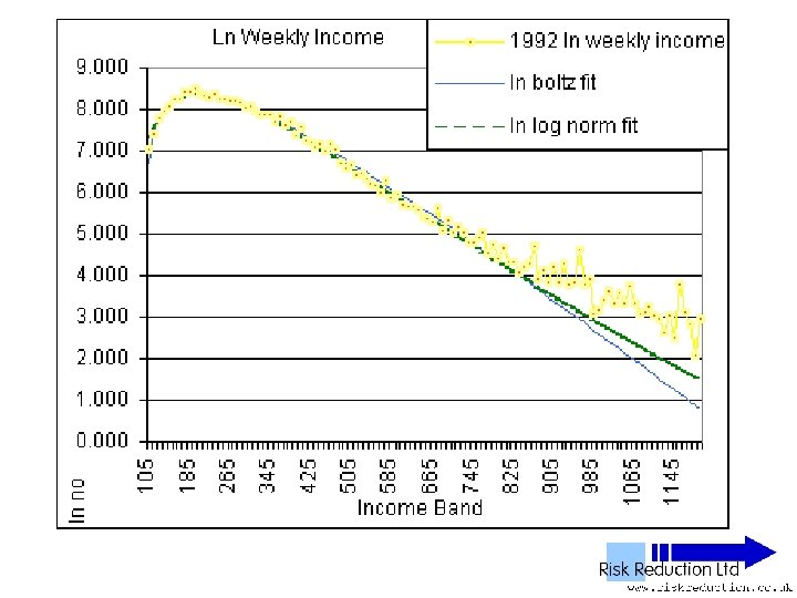
Income Distributions - History • Assumed log-normal - but not derived from economic theory • Known power tail – Pareto - 1896 - strongly demonstrated by Souma Japan data - 2001
Income Distributions - Alternatives • Proposed Exponential - Yakovenko & Dragelescu – US data • Proposed Boltzmann - Willis – 1993 – New Scientist letters • Proposed Boltzmann - Mimkes & Willis – Theortetical derivation - 2002
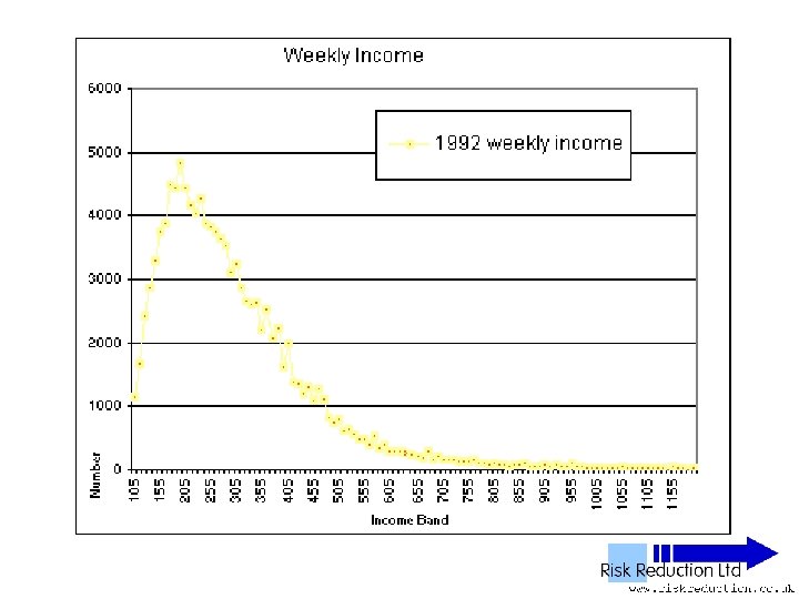
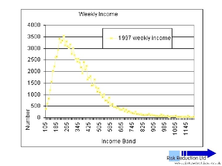
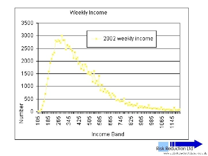
UK NES Data • • • ‘National Earnings Survey’ United Kingdom National Statistics Office Annual Survey 1% Sample of all employees 100, 000 to 120, 000 in yearly sample
UK NES Data • • • 11 Years analysed 1992 to 2002 inclusive 1% Sample of all employees 100, 000 to 120, 000 in yearly sample Wide – PAYE ‘Pay as you earn’ Excludes unemployed, self-employed, private income & below tax threshold “unwaged”
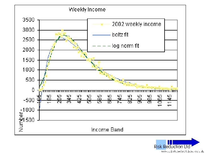
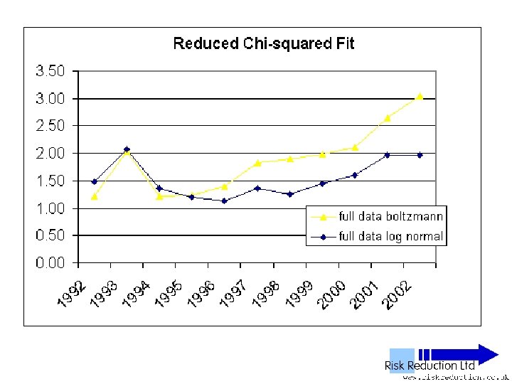
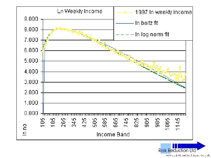
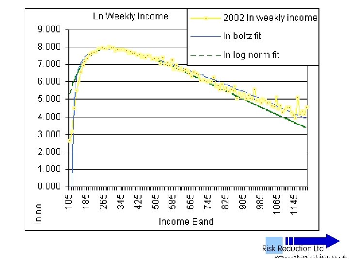
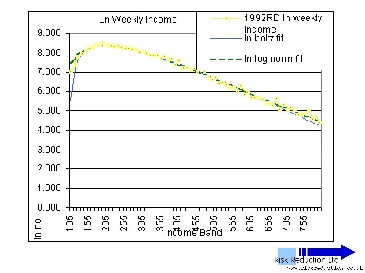
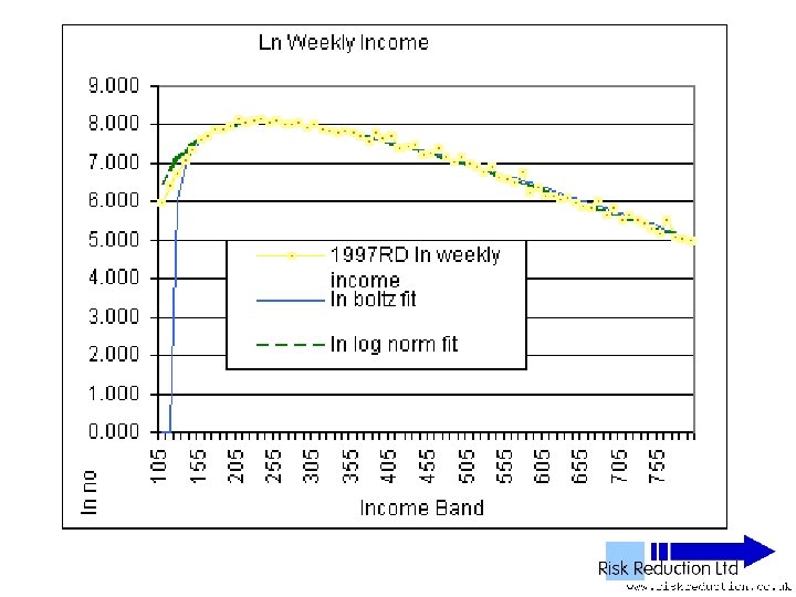
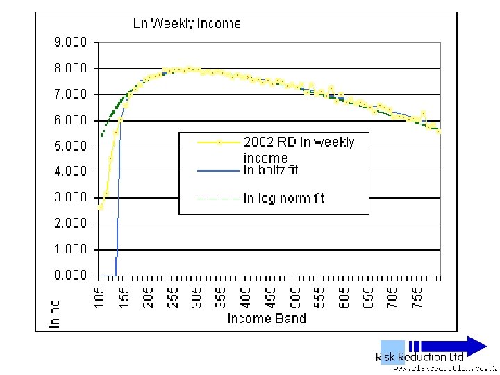
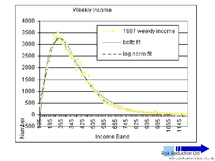
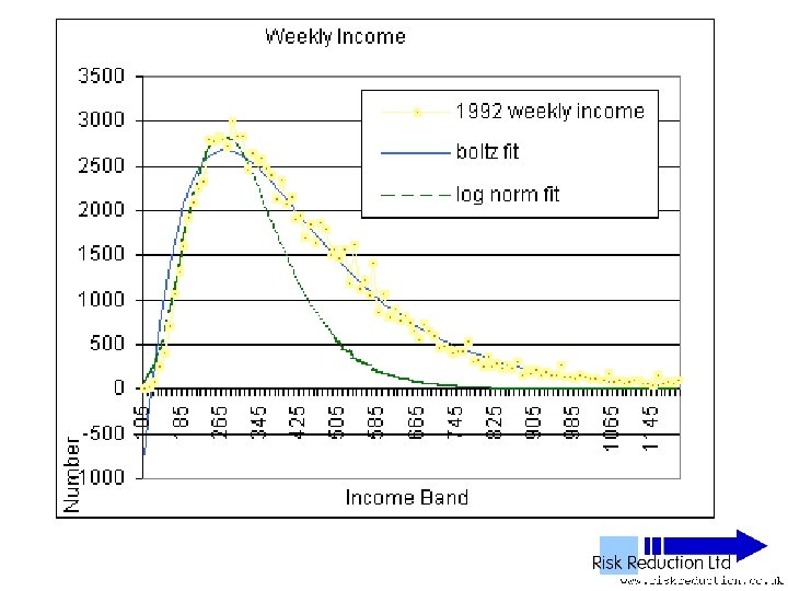
Three Parameter Fits • Used Solver in Excel to fit two functions: • Log-normal F(x) = A*(EXP(-1*((LN(x)-M)))/(2*S*S)))/((x)*S*(2. 5066)) Parameters varied: A, S & M
Three Parameter Fits • Used Solver in Excel to fit two functions: • Boltzmann F(x) = B*(x-G)*(EXP(-P*(x-G))) Parameters varied: B, P & G
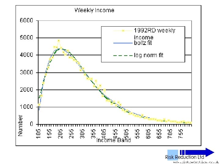
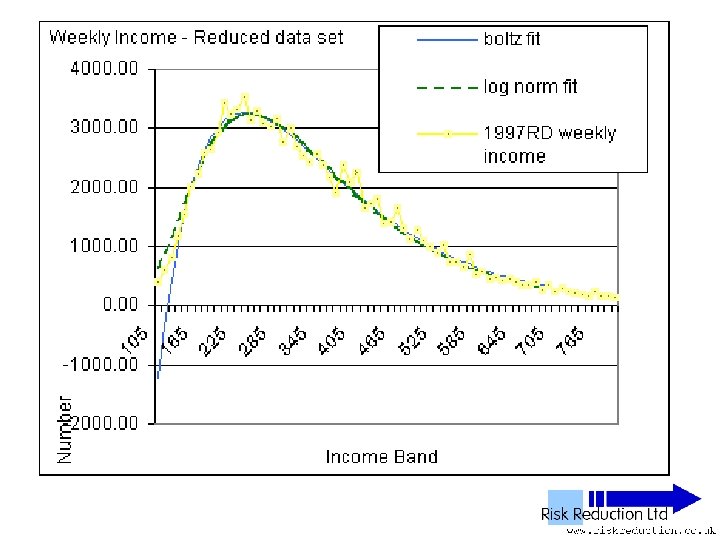
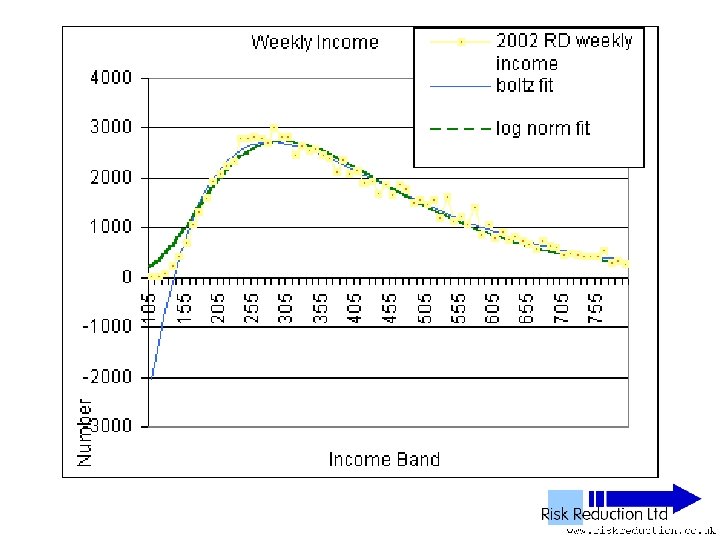
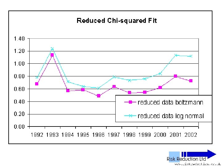
Reduced Data Sets • Deleted data above £ 800 • Deleted data below £ 130 • Repeated fitting of functions
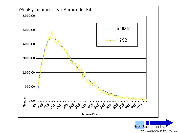
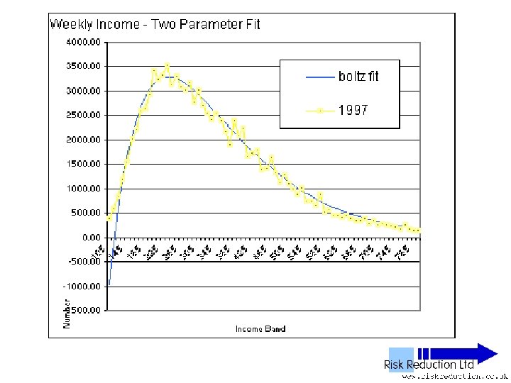
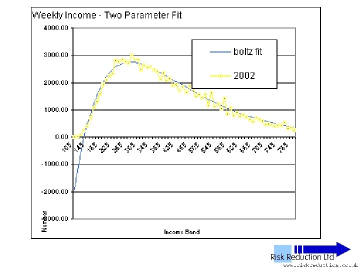
Two Parameter Fits • Boltzmann function only • Reduced Data Set F(x) =B*(x-G)*(EXP(-P*(x-G))) It can be shown that: B =10*No*P*P where No is the total sum of people (factor of 10 arises from bandwidth of data: £ 101£ 110 etc)
Two Parameter Fits • Boltzmann function, Red Data Set F(x) =B*(x-G)*(EXP(-P*(x-G))) B =10*No*P*P So: F(x) =10*No*P*P*(x-G)*(EXP(-P*(x-G))) Parameters varied: P & G only
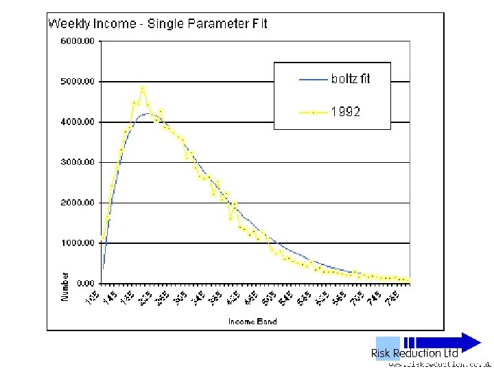
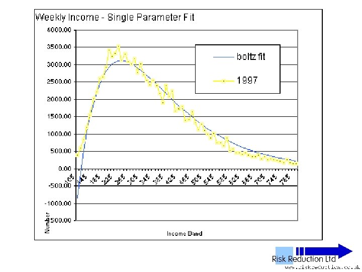
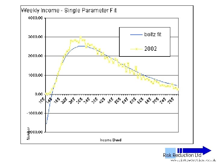
One Parameter Fits • Boltzmann function, Reduced Data Set F(x) =10*No*P*P*(x-G)*(EXP(-P*(x-G))) Parameters varied: P & G only • It can be further shown that: P =2 / (Ko/No – G) where Ko is the total sum of people in each population band multiplied by average income of the band • Note that Ko Will be overestimated due to extra wealth from power tail
One Parameter Fits • Boltzmann function analysed only • Fitted to Reduced Data Set F(x) = B*(x-G)*(EXP(-P*(x-G))) • Can be re-written as: F(x) =10*No*(2/((Ko/No)-G))*(x-G)*(EXP(-(2/((Ko/Pop)-G))*(x-G))) Parameter varied: G only
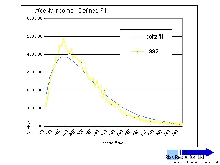
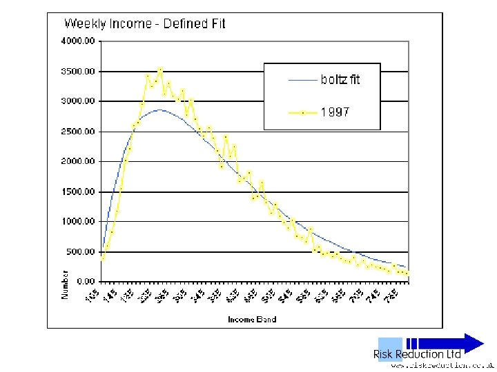
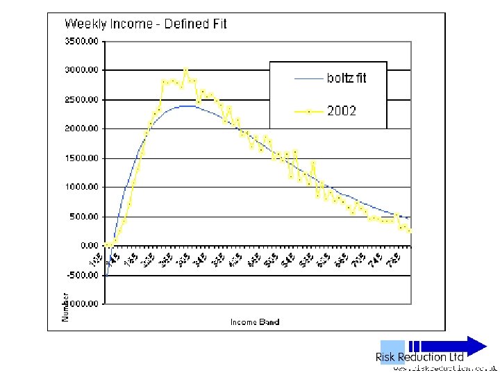
Defined Fit can be calculated from the raw data • G is the offset - can be derived from the raw data - by graphical interpolation Used solver for simple linear regression, 1 st 6 points 1992, 1 st 12 points 1997 & 2002 • Ko & No
Defined Fit • Used function: F(x) =10*No*(2/((Ko/No)-G))*(x-G)*(EXP(-(2/((Ko/Pop)-G))*(x-G))) • Parameter No derived from raw data • Parameter Ko derived from raw data • Parameter G extrapolated from graph of raw data Inserted Parameter into function and plotted results
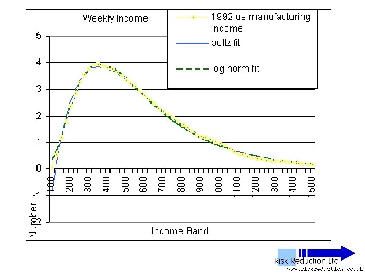
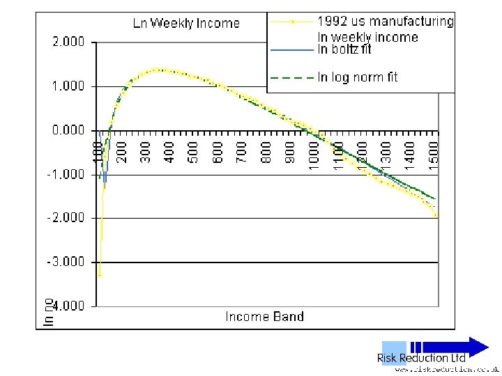
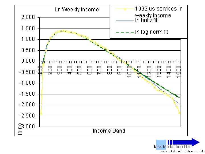
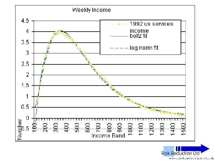
US Income data • Ultimate source: US Department of Labor, Bureau of Statistics • Believed to be good provenance • Details of sample size not know • Details of sampling method not know
US Income data • Note: No power tail Data drops down, not up Believed to be detailed comparison of manufacturing income versus services income • Assumed that only waged income was used
Malleability of log-normal • Un-normalised log-normal F(x) = A*(EXP(-1*((LN(x)-M)))/(2*S*S)))/((x)*S*(2. 5066)) is a three parameter function • A - size • M - offset • S - skew
More Theory • Mimkes & Willis – Boltzmann distribution • Souma & Nirei – this conference • Simple explanation for power law, Allows saving Requires exponential base
Modelling • Chattarjee, Chakrabati, Manna, Das, Yarlagadda etc • Have demonstrated agent models that: – give exponential results (no saving) – give power tails (saving allowed)
Conclusions • Evidence supports: Boltzmann distribution low / medium income Power law high income • Theory supports: Boltzmann distribution low / medium income Power law high income • Modelling supports: Boltzmann distribution low / medium income Power law high income
Geoff Willis