GENETIC ALGORITHMS One semester graduate course Prof Boris

GENETIC ALGORITHMS One semester graduate course Prof. Boris Epstein The Academic College of Tel-Aviv-Yaffo 1

Outline • • • Introduction to Genetic Algorithms (GAs) Theoretical Foundations Computer Implementation of GAs Applications of GAs Advanced Techniques and Applications 2

Part I SHORT SURVEY OF OPTIMIZATION METHODS • • What is it About Basic Approaches GAs: Basic Features Conventional Optimization Methods vs. GAs 3

OPTIMIZATION: The search for the best solution among alternatives, or the extreme value of a function f The function f is called an objective function, or cost function. A feasible solution that minimizes (or maximizes, if that is the goal) the objective function is called an optimal solution 4

Overview of conventional search methods • Calculus-based methods (Gradient methods) • Enumerative methods (like dynamic programming) • Random methods and semi-random methods (like simulated annealing) 5

Conventional search methods: Calculus-based methods (1) • Gradient (vector of partial derivatives) of the objective function is set to zero • In the case of a function defined analytically, this may be done explicitly • Otherwise, the function is climbed (or descended) in the steepest possible direction. Iteratively, after calculating the gradient (exactly or approximately), a finite step is performed in the gradient direction. 6

Conventional search methods: Calculus-based methods (2) • Local in scope (a multiple-peak function causes a problem: which peak to climb? ) • Require smoothness (derivatives). Real-life data are sometimes discontinuous and noisy! • Constraints are not easy to impose as an optimum often resides on the constraints boundary • Lack of robustness 7

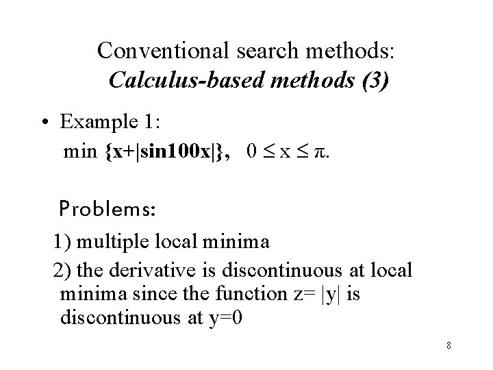
Conventional search methods: Calculus-based methods (3) • Example 1: min {x+|sin 100 x|}, 0 x π. Problems: 1) multiple local minima 2) the derivative is discontinuous at local minima since the function z= |y| is discontinuous at y=0 8

Conventional search methods: Calculus-based methods (4) • Example 2: minimize {f(x, y, z)} under the constraint 0 g(x, y, z), where 0 x 1, 0 y 1, 0 z 1, and the function g(x, y, z) is defined as a black-box which contains numerical noise. How to calculate the gradient (derivatives) accurately? 9

Conventional search methods: Enumerative methods • Check every point within a finite search space. • Practical problems are too large to search one at a time. • “Curse of dimensionality”: break down on problems of moderate size and complexity. • Lack of efficiency 10

Conventional search methods: Dynamic Programming (1) A sophisticated example: dynamic programming. The problem can be • • • ` divided into stages with a decision required at each stage. Each stage has a number of states associated with it. The decision at one stage transforms one state into a state in the next stage. Principal of optimality: Given the current state, the optimal decision for each of the remaining states does not depend on the previous states or decisions. There exists a recursive relationship that identifies the optimal decision for stage j, given that stage j+1 has already been solved. The final stage must be solvable by itself. • It is an art to determine stages and states. 11

Conventional search methods: Dynamic Programming (2) • A corporation has $5 million to allocate to its three plants for possible expansion. • Each plant has submitted a number of proposals specifying (i) the cost of the expansion c and (ii) the total revenue expected r. • Each plant is only permitted to realize one of its proposals. • The goal is to maximize the firm’s revenues resulting from the allocation of the $5 million. 12

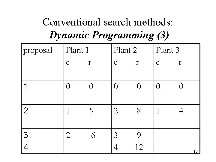
Conventional search methods: Dynamic Programming (3) proposal Plant 1 c r Plant 2 c r Plant 3 c r 1 0 0 2 1 5 2 8 1 4 3 4 2 6 3 9 4 12 13

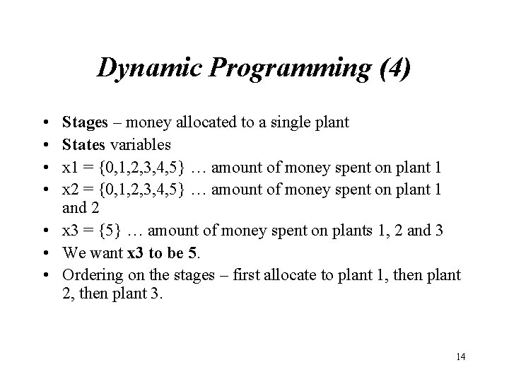
Dynamic Programming (4) • • Stages – money allocated to a single plant States variables x 1 = {0, 1, 2, 3, 4, 5} … amount of money spent on plant 1 x 2 = {0, 1, 2, 3, 4, 5} … amount of money spent on plant 1 and 2 • x 3 = {5} … amount of money spent on plants 1, 2 and 3 • We want x 3 to be 5. • Ordering on the stages – first allocate to plant 1, then plant 2, then plant 3. 14

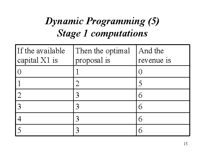
Dynamic Programming (5) Stage 1 computations If the available capital X 1 is 0 1 2 3 Then the optimal proposal is 1 2 3 3 And the revenue is 0 5 6 6 4 5 3 3 6 6 15

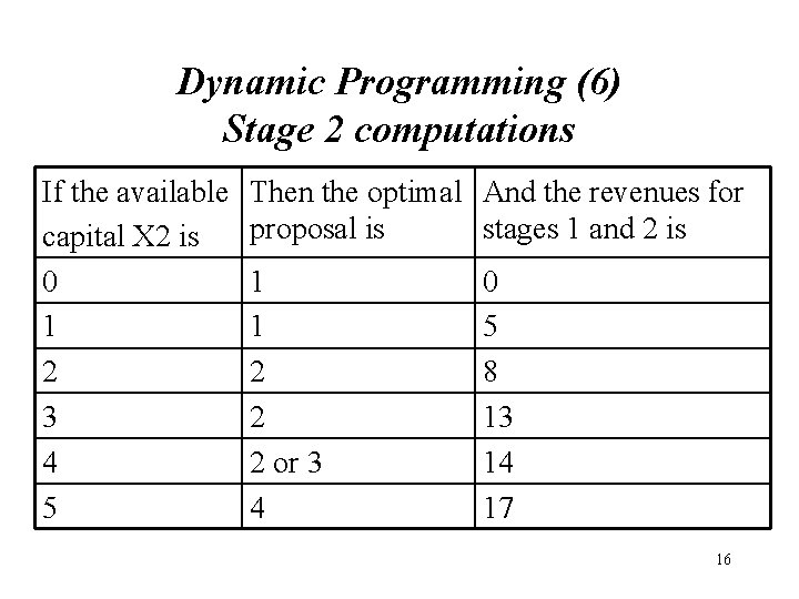
Dynamic Programming (6) Stage 2 computations If the available capital X 2 is 0 1 2 3 4 5 Then the optimal And the revenues for proposal is stages 1 and 2 is 1 1 2 2 2 or 3 4 0 5 8 13 14 17 16

Dynamic Programming (7) Example : Determine the best allocation for state x 2=4 1. Proposal 1 gives revenue of 0, leaves 4 for stage 1, which returns 6. Total=6. 2. Proposal 2 gives revenue of 8, leaves 2 for stage 1, which returns 6. Total=14. 3. Proposal 3 gives revenue of 9, leaves 1 for stage 1, which returns 5. Total=14. 4. Proposal 4 gives revenue of 12, leaves 0 for stage 1, which returns 0. Total=12. 17

Dynamic Programming (8) • Stage 3 computations, we are interested in x 35= • . 1 Proposal 1 gives revenue 0, leaves 5. Previous stages give 17. Total=17. • . 2 Proposal 2 gives revenue 4, leaves 4. Previous stages give 14. Total=18. • The optimal solution, that gives a revenue 18, is to implement • - proposal 2 at plant 3 , • - proposal 2 or 3 at plant 2, and • - proposal 3 or 2 at plant 1. 18

Conventional search methods: Enumerative methods (4) For the Traveling Salesman Problem (TSP), let stage m represent visiting m cities (of total N) and let the decision be where to go next. The salesman starts and finishes in city #1. A state is represented by a pair (n, S) where S is the set of m cities already visited and n S is the last city visited. Denoting cij the distance between cities i and j, we get a backward recursion: fm(i, S) = min{cij+fm+1(j, S j)} over j S, and, on the stage N-1, decisions are easily calculated. Problem of dimensionality: for 30 cities, the number of states in the 15 th stage is more than a billion! 19

Conventional search methods: Random methods (1) A simple example: Monte Carlo Simulation (MCS) which represents a large number of random trials. Information is obtained by tabulating the results of these trials. E. g. , you determine the probability of flipping a coin and having it land on heads if the coin initially starts with the heads-face showing. The MCS have you flip the coin a large number of times, each time with heads showing before you flip, and recording the number of times the coin lands on heads. The number of times it lands on heads divided by the total number of times the coin is flipped yields the probability of getting heads if you start from heads. 20

Conventional search methods: Random methods (2) Random search: search randomly as much as you can and save the best Strictly random methods do better than enumerative search but still are not sufficiently efficient. • Random search is a strategy which exploits the search space but ignores the exploitations of the promising regions of the space. • Randomized technique: random choice as a tool in a directed search process. 21

Conventional search methods: Random methods (3) Example of randomized technique: Simulated annealing which uses random approach in search for minimal energy states. The idea: a probability p of acceptance (i. e. replacement of the current point by a new one) is 1 if the new point provides a better value of the objective function but p > 0 otherwise! The probability p is a function of the values of objective function for the current point and the new point and “temperature” T. The lower T is, the smaller p, and during execution of the algorithm, T is lowered by steps. 22

Conventional search algorithms: main drawbacks • Many traditional methods work good in a narrow problem domain. • Enumerative schemes and random walks are inefficient across the broad spectrum. • GAs: in the quest of robustness and efficiency. 23

GAs: overview According to Darwin, life is a struggle in which only the fittest survive to reproduce. What has proved successful to life is also useful to problem solving on a computer. Programs using so-called genetic algorithms find solutions by applying the strategies of natural selection. The algorithm first advances possible answers. Then, like biological organisms, the solutions "cross over, " or exchange "genes, " with every generation. Sometimes there are mutations, or changes, in the genes. Only the "fittest" solutions survive so that they can reproduce to create even better answers. 24

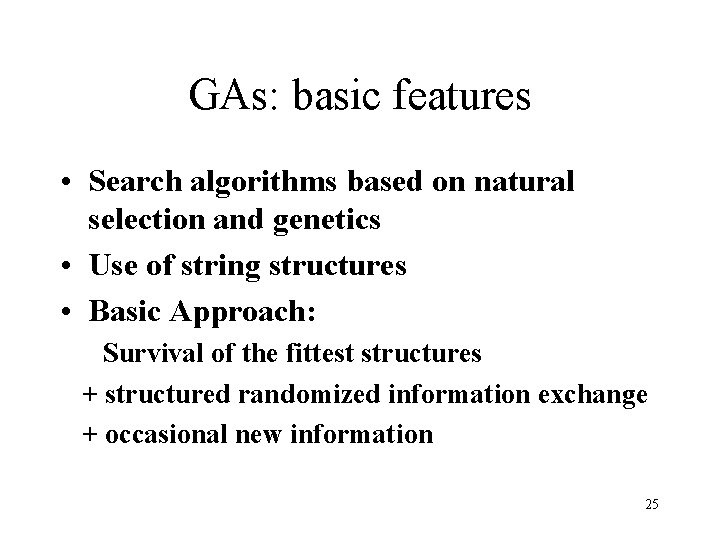
GAs: basic features • Search algorithms based on natural selection and genetics • Use of string structures • Basic Approach: Survival of the fittest structures + structured randomized information exchange + occasional new information 25

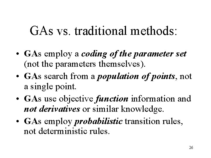
GAs vs. traditional methods: • GAs employ a coding of the parameter set (not the parameters themselves). • GAs search from a population of points, not a single point. • GAs use objective function information and not derivatives or similar knowledge. • GAs employ probabilistic transition rules, not deterministic rules. 26

Part II Introduction to Genetic Algorithms • • Basic Approach Basic Components Genetic Operators Simulation by hand 27

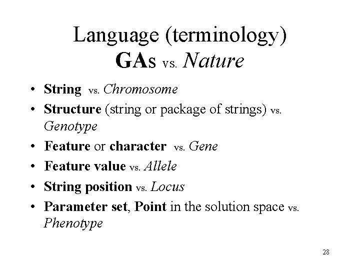
Language (terminology) GAs vs. Nature • String vs. Chromosome • Structure (string or package of strings) vs. Genotype • Feature or character vs. Gene • Feature value vs. Allele • String position vs. Locus • Parameter set, Point in the solution space vs. Phenotype 28

Basic Approach (1) A population of abstract representations of candidate solutions (individuals) to an optimization problem evolves toward better solutions. Traditionally, solutions are represented in binary as strings of 0 s and 1 s, but other encodings are also possible. The evolution usually starts from a population of randomly generated individuals and happens in generations. 29

Basic Approach (2) In each generation, the fitness of every individual in the population is evaluated, multiple individuals are stochastically selected from the current population (based on their fitness), and modified (recombined and possibly randomly mutated) to form a new population. The new population is then used in the next iteration of the algorithm. Commonly, the algorithm terminates when either a maximum number of generations has been produced, or a satisfactory fitness level has been reached for the population. 30

Basic Approach (3) A typical genetic algorithm requires three things to be defined: • a genetic representation of the solution domain • An objective (fitness) to evaluate the solution domain • Genetic operators: selection, crossover, mutation 31

GAs: Basic components • Coding (a genetic representation for potential solutions to the problem). • Creation of an initial population of potential solutions. • An evaluation function (objective function) that rates solution in terms of their fitness. • An operator that selects a “mating pool” (“Selection”). • Genetic operators that alter the composition of “children” (“Crossover” and “Mutation”). • Values for various parameters of the GA: population size, probabilities of applying genetic operator etc. . 32

GAs: Coding • Coding is a genetic representation for solutions to the problem. • The solutions are represented as finite strings over a finite alphabet. The simplest and a very important case: binary coding (the coding over the alphabet {0, 1}). In this case, each string consists of 0’s and 1’s. • In numerical optimization, float-point coding is frequently used. • Structures more complicated than strings may be also employed. 33

GAs: Initial population and subsequent generations • Initial population (the first generation) is generated randomly. • It is possible to seed a few deterministically chosen representatives in an initial population but in most problems this is redundant and may even to slow down the convergence. • Subsequent generations are generated iteratively by 1) Evaluation of the current population 2) Selection of “parents” according to their fitness 3) Choice of mates 4) Crossover and mutation 34

GAs: Evaluation • Each string is evaluated by means of an objective function. • The objective function evaluates numerically the fitness of solution. This may be a “black box”-type function, analytical function, table of values etc. • An evaluation function must be positive (nonnegative). If necessary, it is transformed to a fitness form by a transformation. • A crucial requirement to fitness function: to preserve the relation of order over the population. 35

GAs: Reproduction (Selection of mating pool (1)) • This is the first step in generating a new population. • Selection of a “mating pool” is performed by a special operator. • The operator selects a number of representatives from a current population favoring the fittest strings and discriminating the less fit. Different operators are available: roulette-type selection, tournament selection etc. • More fit strings may provide several representatives to the pool, and less fit strings may “die”. 36

GAs: Reproduction (Selection of mating pool (2)) • Roulette-type selection: Allocation of strings using a roulette wheel with slots sized according to relative fitness of strings. • More fit strings may provide several representatives to the pool, and less fit strings may “die”. 37

GAs: Reproduction (Selection of mating pool (3)) Tournament selection: Random pairs play “tournaments” in such a way that a more fit string has higher probability to be included into the mating pool. E. g. , for each pair, a uniformly distributed random number between 0 and 1 is generated. If the random value is less than a prescribed value PV >>. 5 then a more fit string joins the pool. Otherwise a less fit string is included. 38

GAs: Choice of mates • A mating pool is randomly subdivided into pairs. • First, each pair produces two “children” by a simple reproduction of both parents. Remind that some “parents” may be duplicated in the pool and thus are reproduced more than once. • On the next stage, the reproduced strings are changed by a crossover (see the next slide). • Finally, a low-rate mutation operator may randomly change some bits in the new strings. 39

GAs: Crossover • Crossover operator performs exchange of string characters (bits for binary strings) according to the choice of a crossover site(s). • A crossover site is usually chosen randomly for each pair. • In a simple crossover, a crisscross exchange of bits is applied. In a multiple crossover, several positions are specified as the crossover cites which multiplies the possibilities for the exchange. • More fancy crossover operators may be easily produced. 40

GAs: Mutation • Mutation randomly changes bits following the crossover, according to the mutation rate. • Mutation is a tool of diversifying the population in a random way. • Mutation allows to explore the combinations of bits not present in their parents. (E. g. if the parents are identical, a crossover is reduced to a simple reproduction). • Usually the mutation rate is taken low (. 001 -. 05). 41

GAs: Convergence • After a GA has run for many generations, most of the population consists of very similar strings. This is called convergence and occurs because the genetic algorithm pushes the population into ever narrower target regions. • Sometimes the population will converge to an individual that is not the optimal one (a local optimum found). In this case, the crossover will not contribute much to the search for better individuals as crossing two identical strings will yield the same two strings, so nothing new happens. One possible mechanism to repair this is to bias the selection process to keep the population diverse. 42

A simple genetic algorithm: simulation by hand (1) • Maximize F(x)=x 2 , x=0, 1, 2, …. , 31. • Coding: binary unsigned of length 5. • Initial population : randomly generated (e. g. 4 repetitions of 5 coin tosses). • Calculate the fitness of the population. • Reproduction (selection of a “mating pool”) according to fitness. It may be simulated by spinning a roulette wheel with slots sized according to fitness. 43

A simple genetic algorithm: simulation by hand (2) • • Selection of mates (randomly selected). Selection of crossover site (randomly selected). Crossover (new population created). Mutation (change of the new population according a chosen rate of mutation) • Calculate the fitness of the new population. • A new generation is treated as the initial one: reproduction, selection of mates, crossover, mutation, ……. 44

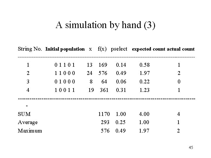
A simulation by hand (3) String No. Initial population x f(x) pselect expected count actual count --------------------------------------------------- 1 0 1 1 0 1 13 169 0. 14 0. 58 1 2 1 1 0 0 0 24 576 0. 49 1. 97 2 3 0 1 0 0 0 8 64 0. 06 0. 22 0 4 1 0 0 1 1 19 361 0. 31 1. 23 1 ---------------------------------------------SUM 1170 1. 00 4. 00 4 Average 293 0. 25 1. 00 1 Maximum 576 0. 49 1. 97 2 45

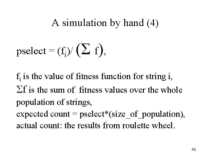
A simulation by hand (4) pselect = (fi)/ (Σ f), fi is the value of fitness function for string i, Σf is the sum of fitness values over the whole population of strings, expected count = pselect*(size_of_population), actual count: the results from roulette wheel. 46

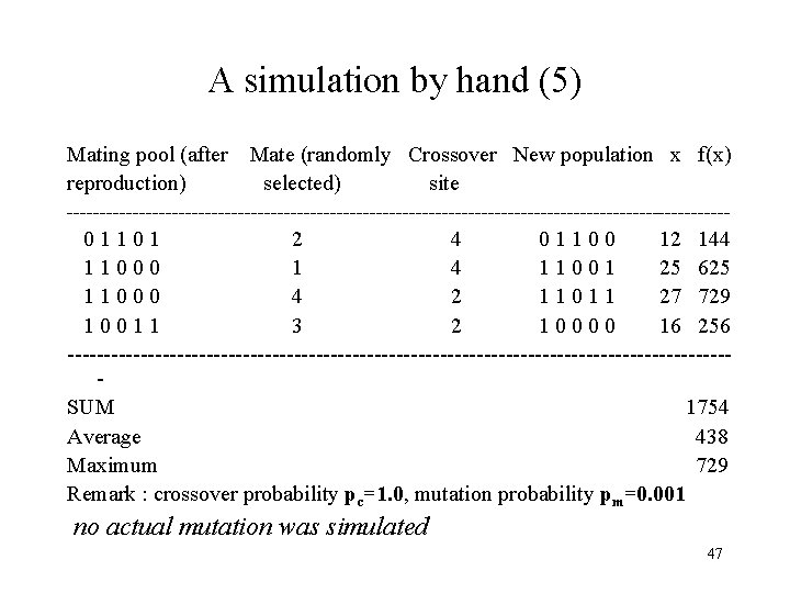
A simulation by hand (5) Mating pool (after Mate (randomly Crossover New population x f(x) reproduction) selected) site --------------------------------------------------- 0 1 1 0 1 2 4 0 1 1 0 0 12 144 1 1 0 0 0 1 4 1 1 0 0 1 25 625 1 1 0 0 0 4 2 1 1 0 1 1 27 729 1 0 0 1 1 3 2 1 0 0 16 256 ---------------------------------------------SUM 1754 Average 438 Maximum 729 Remark : crossover probability pc=1. 0, mutation probability pm=0. 001 no actual mutation was simulated 47

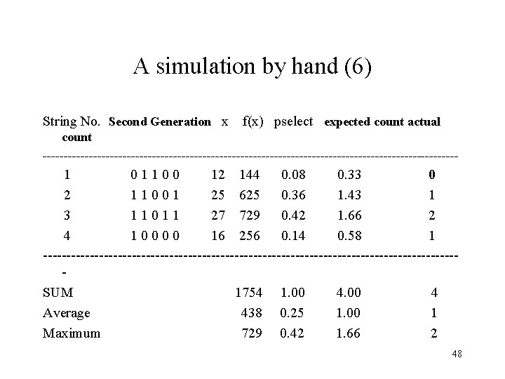
A simulation by hand (6) String No. Second Generation x f(x) pselect expected count actual count -------------------------------------------------- 1 0 1 1 0 0 12 144 0. 08 0. 33 0 2 1 1 0 0 1 25 625 0. 36 1. 43 1 3 1 1 0 1 1 27 729 0. 42 1. 66 2 4 1 0 0 16 256 0. 14 0. 58 1 --------------------------------------------SUM 1754 1. 00 4. 00 4 Average 438 0. 25 1. 00 1 Maximum 729 0. 42 1. 66 2 48

A simulation by hand (7) Mating pool (after Mate (randomly Crossover New population x f(x) reproduction) selected) site --------------------------------------------------- 1 1 0 0 1 3 1 1 0 1 1 27 729 1 1 0 1 1 4 1 1 0 26 676 1 1 0 1 1 3 1 1 0 0 1 25 625 1 0 0 2 4 1 0 0 0 1 17 289 ----------------------------------------------SUM 2319 Average 580 Maximum 729 Remark : crossover probability pc=1. 0, mutation probability pm=0. 001 no actual mutation was simulated 49

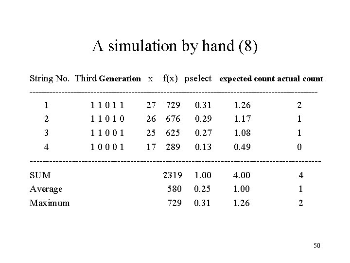
A simulation by hand (8) String No. Third Generation x f(x) pselect expected count actual count -------------------------------------------------- 1 1 0 1 1 27 729 0. 31 1. 26 2 2 1 1 0 26 676 0. 29 1. 17 1 3 1 1 0 0 1 25 625 0. 27 1. 08 1 4 1 0 0 0 1 17 289 0. 13 0. 49 0 ---------------------------------------------SUM 2319 1. 00 4. 00 4 Average 580 0. 25 1. 00 1 Maximum 729 0. 31 1. 26 2 50

A simulation by hand (9) Mating pool (after Mate (randomly Crossover New population x f(x) reproduction) selected) site --------------------------------------------------- 1 1 0 1 1 2 1 1 0 1 1 27 729 1 1 0 1 1 1 1 0 1 1 27 729 1 1 0 4 1 1 0 1 1 27 729 1 1 0 0 1 3 4 1 1 0 0 0 24 576 ----------------------------------------------SUM 2763 Average 691 Maximum 729 Remark : crossover probability pc=1. 0, mutation probability pm=0. 001 no actual mutation was simulated 51

A simulation by hand (8): discussion of the first two iterations • Population is rapidly improving. • Maximum value will remain 27 (and not the optimal 31) which may be (hopefully) improved by a greater rate of mutation. Without a mutation, the value of the middle bit will remain zero forever! • The initial population was not diversified enough – much more greater populations are needed. 52

Part III Implementation of a simple GA • How to implement a simple GA • Sample problem 53

Implementation of a simple GA (1) • First step: write the utilities to make the program easy to run, to change parameter settings and to display the population and statistics about its performance. • Second step: to track the population's average fitness and the most fit members of each generation. The program should generate random populations of individuals and have subroutines to assign fitness. The program should also display the individuals and their fitness, sort by fitness and calculate the average fitness of the population. 54

Implementation of a simple GA (2) • Third step: write subroutines to implement the genetic algorithm itself. That is, your program should select parents from the current population and modify the offspring of those parents through crossover and mutation. • The Evaluate. Population subroutine simply loops over all the individuals in the population, assigning each an f(x) value as a measure of fitness. The Do. Tournament. Selection subroutine conducts a series of tournaments between randomly selected individuals and usually, but not always, copies the fittest individual of the pair (i, , j) to New. Pop. 55

Implementation of a simple GA (3) • In a sample tournament selection algorithm, URand 01 returns a (uniformly distributed) random value between 0 and 1. More fit individuals tend to have more off-springs in the new population than do less fit ones. • It is sometimes useful to copy the fittest individual into the new populations every generation (the elitism principle). • If URand 01 is greater than 0. 75, the selective pressure will be greater (it will be harder for less fit strings to be copied into New. Pop), whereas a smaller value will yield less selective pressure. If 0. 5 is used, there will be no selective pressure at all. 56

Implementation of a simple GA (4) • The Modify. Population subroutine should randomly perform the crossover operation on some of the pairs in New. Pop, a typical crossover rate is 0. 75 (that is, cross 75 percent of the pairs). The simplest crossover is the "single point" crossover operation. • The Mutate. Population mutates a small, randomly selected number of bits in the individual strings, changing the value from 1 to 0, or vice versa. A typical mutation rate is 0. 005 -0. 03 per bit, that is, in the case of a 0. 005 rate, each bit has a 0. 005 chance of being mutated. 57

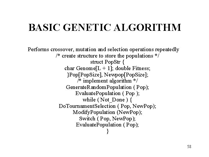
BASIC GENETIC ALGORITHM Performs crossover, mutation and selection operations repeatedly /* create structure to store the populations */ struct Pop. Str { char Genome[L + 1]; double Fitness; }Pop[Pop. Size], Newpop[Pop. Size]; /* implement algorithm */ Generate. Random. Population ( Pop); Evaluate. Population ( Pop ); while ( Not_Done ) { Do. Tournament. Selection ( Pop, New. Pop); Modify. Population (New. Pop); Switch ( Pop, New. Pop); Evaluate. Population ( Pop); } 58

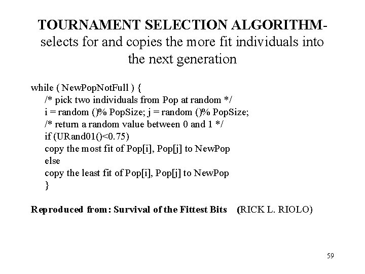
TOURNAMENT SELECTION ALGORITHMselects for and copies the more fit individuals into the next generation while ( New. Pop. Not. Full ) { /* pick two individuals from Pop at random */ i = random ()% Pop. Size; j = random ()% Pop. Size; /* return a random value between 0 and 1 */ if (URand 01()<0. 75) copy the most fit of Pop[i], Pop[j] to New. Pop else copy the least fit of Pop[i], Pop[j] to New. Pop } Reproduced from: Survival of the Fittest Bits (RICK L. RIOLO) 59

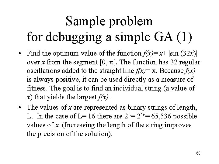
Sample problem for debugging a simple GA (1) • Find the optimum value of the function f(x)= x+ |sin (32 x)| over x from the segment [0, p]. The function has 32 regular oscillations added to the straight line f(x)= x. Because f(x) is always positive, it can be used directly as a measure of fitness. The goal is to find an individual string (a value of x) that yields the largest f(x). • The values of x are represented as binary strings of length, L. In the case of L= 16 there are 2 L= 216= 65, 536 possible values of x. (Increasing the length of the string improves the precision of the solution). 60

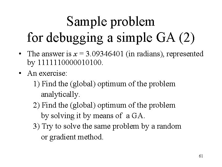
Sample problem for debugging a simple GA (2) • The answer is x = 3. 09346401 (in radians), represented by 1111110000010100. • An exercise: 1) Find the (global) optimum of the problem analytically. 2) Find the (global) optimum of the problem by solving it by means of a GA. 3) Try to solve the same problem by a random or gradient method. 61

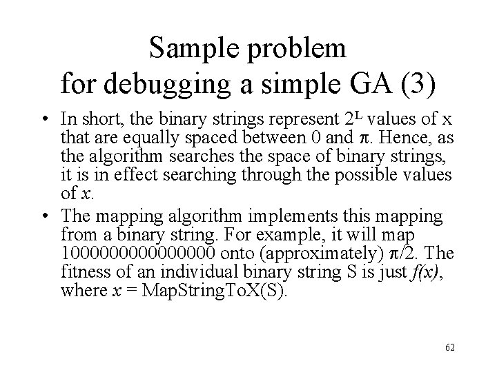
Sample problem for debugging a simple GA (3) • In short, the binary strings represent 2 L values of x that are equally spaced between 0 and p. Hence, as the algorithm searches the space of binary strings, it is in effect searching through the possible values of x. • The mapping algorithm implements this mapping from a binary string. For example, it will map 100000000 onto (approximately) p/2. The fitness of an individual binary string S is just f(x), where x = Map. String. To. X(S). 62

Part IV Similarity Templates • • Interaction between crossover and coding Schemata Building block hypothesis Simulation by hand revisited 63

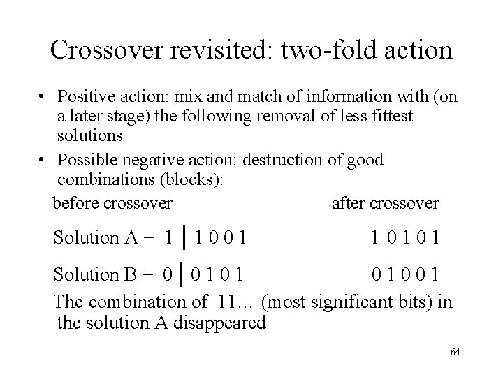
Crossover revisited: two-fold action • Positive action: mix and match of information with (on a later stage) the following removal of less fittest solutions • Possible negative action: destruction of good combinations (blocks): before crossover after crossover Solution A = 1 | 1 0 0 1 1 0 1 Solution B = 0 | 0 1 0 1 0 0 1 The combination of 11… (most significant bits) in the solution A disappeared 64

Interaction of coding and crossover (1) • Is the type of coding really important? • How this effects the crossover? • Example: Consider a different coding for the exercise on slides 43 -52 (maximize F(x)=x 2, x=0, 1, 2, …. , 31). The previous coding: binary unsigned of length 5. 65

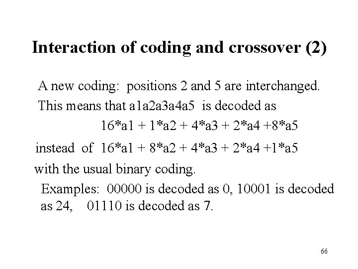
Interaction of coding and crossover (2) A new coding: positions 2 and 5 are interchanged. This means that a 1 a 2 a 3 a 4 a 5 is decoded as 16*a 1 + 1*a 2 + 4*a 3 + 2*a 4 +8*a 5 instead of 16*a 1 + 8*a 2 + 4*a 3 + 2*a 4 +1*a 5 with the usual binary coding. Examples: 00000 is decoded as 0, 10001 is decoded as 24, 01110 is decoded as 7. 66

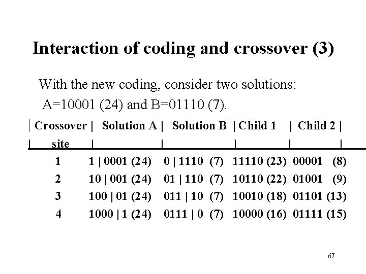
Interaction of coding and crossover (3) With the new coding, consider two solutions: A=10001 (24) and B=01110 (7). | Crossover | Solution A | Solution B | Child 1 | Child 2 | | site 1 2 3 4 | | 1 | 0001 (24) 0 | 1110 10 | 001 (24) 01 | 110 100 | 01 (24) 011 | 10 1000 | 1 (24) 0111 | 0 (7) (7) | | | 11110 (23) 00001 (8) 10110 (22) 01001 (9) 10010 (18) 01101 (13) 10000 (16) 01111 (15) 67

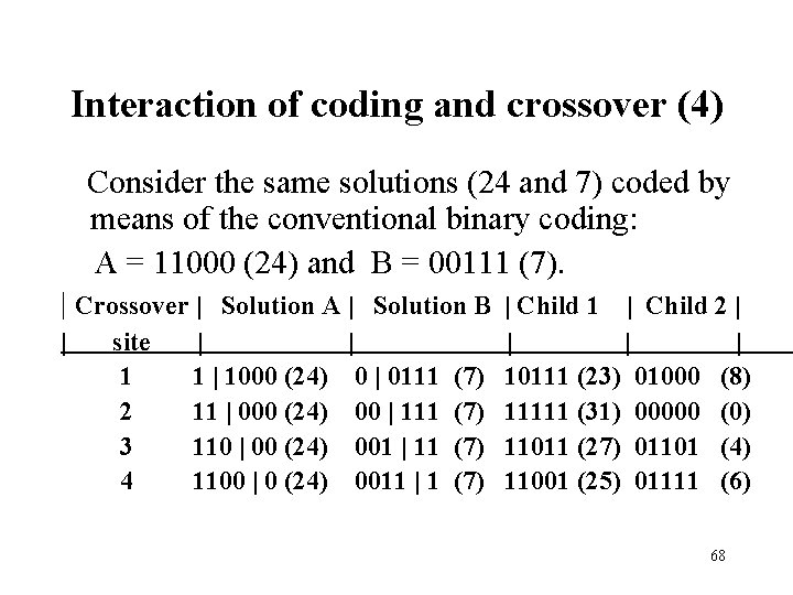
Interaction of coding and crossover (4) Consider the same solutions (24 and 7) coded by means of the conventional binary coding: A = 11000 (24) and B = 00111 (7). | Crossover | Solution A | Solution B | Child 1 | Child 2 | | site 1 2 3 4 | | 1000 (24) 0 | 0111 11 | 000 (24) 00 | 111 110 | 00 (24) 001 | 11 1100 | 0 (24) 0011 | 1 (7) (7) | | 10111 (23) 01000 11111 (31) 00000 11011 (27) 01101 11001 (25) 01111 | (8) (0) (4) (6) 68

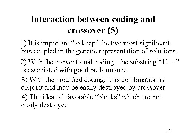
Interaction between coding and crossover (5) 1) It is important “to keep” the two most significant bits coupled in the genetic representation of solutions. 2) With the conventional coding, the substring “ 11…” is associated with good performance 3) With the modified coding, this combination is disjoint and may be easily destroyed by crossover 4) The idea of favorable “blocks” which are not easily destroyed 69

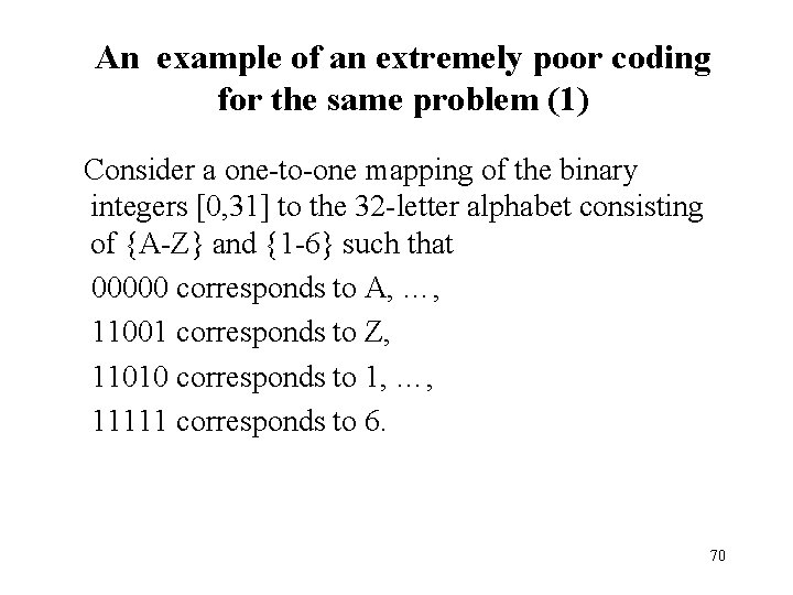
An example of an extremely poor coding for the same problem (1) Consider a one-to-one mapping of the binary integers [0, 31] to the 32 -letter alphabet consisting of {A-Z} and {1 -6} such that 00000 corresponds to A, …, 11001 corresponds to Z, 11010 corresponds to 1, …, 11111 corresponds to 6. 70

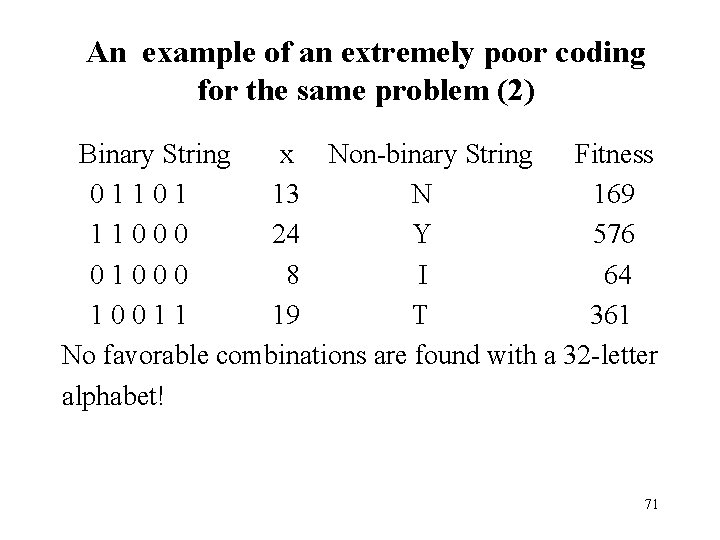
An example of an extremely poor coding for the same problem (2) Binary String x Non-binary String Fitness 0 1 1 0 1 13 N 169 1 1 0 0 0 24 Y 576 0 1 0 0 0 8 I 64 1 0 0 1 1 19 T 361 No favorable combinations are found with a 32 -letter alphabet! 71

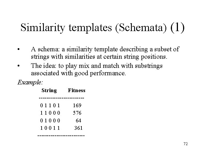
Similarity templates (Schemata) (1) • A schema: a similarity template describing a subset of strings with similarities at certain string positions. • The idea: to play mix and match with substrings associated with good performance. Example: String Fitness ------------ 0 1 1 0 1 169 1 1 0 0 0 576 0 1 0 0 0 64 1 0 0 1 1 361 ------------72

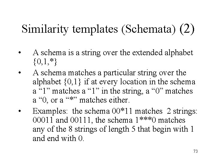
Similarity templates (Schemata) (2) • • • A schema is a string over the extended alphabet {0, 1, *} A schema matches a particular string over the alphabet {0, 1} if at every location in the schema a “ 1” matches a “ 1” in the string, a “ 0” matches a “ 0, or a “*” matches either. Examples: the schema 00*11 matches 2 strings: 00011 and 00111, the schema 1***0 matches any of the 8 strings of length 5 that begin with 1 and end with 0. 73

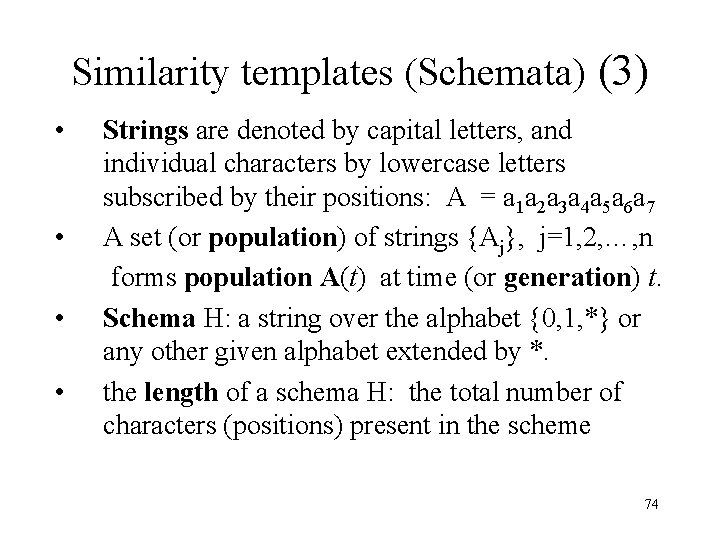
Similarity templates (Schemata) (3) • Strings are denoted by capital letters, and individual characters by lowercase letters subscribed by their positions: A = a 1 a 2 a 3 a 4 a 5 a 6 a 7 • A set (or population) of strings {Aj}, j=1, 2, …, n forms population A(t) at time (or generation) t. • Schema H: a string over the alphabet {0, 1, *} or any other given alphabet extended by *. • the length of a schema H: the total number of characters (positions) present in the scheme 74

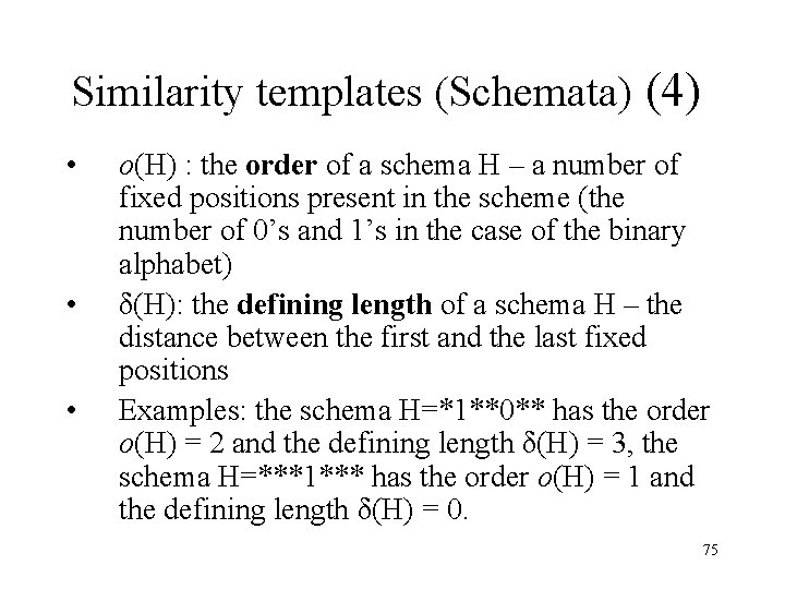
Similarity templates (Schemata) (4) • • • o(H) : the order of a schema H – a number of fixed positions present in the scheme (the number of 0’s and 1’s in the case of the binary alphabet) δ(H): the defining length of a schema H – the distance between the first and the last fixed positions Examples: the schema H=*1**0** has the order o(H) = 2 and the defining length δ(H) = 3, the schema H=***1*** has the order o(H) = 1 and the defining length δ(H) = 0. 75

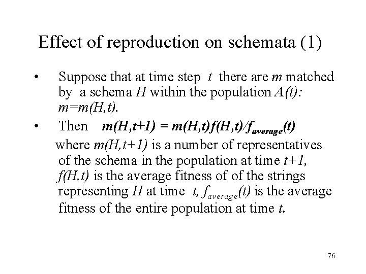
Effect of reproduction on schemata (1) • • Suppose that at time step t there are m matched by a schema H within the population A(t): m=m(H, t). Then m(H, t+1) = m(H, t)f(H, t)/faverage(t) where m(H, t+1) is a number of representatives of the schema in the population at time t+1, f(H, t) is the average fitness of of the strings representing H at time t, faverage(t) is the average fitness of the entire population at time t. 76

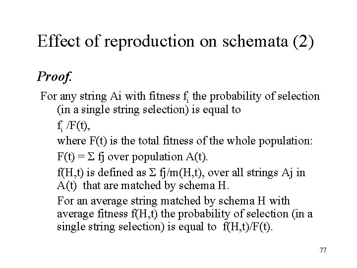
Effect of reproduction on schemata (2) Proof. For any string Ai with fitness fi the probability of selection (in a single string selection) is equal to fi /F(t), where F(t) is the total fitness of the whole population: F(t) = Σ fj over population A(t). f(H, t) is defined as Σ fj/m(H, t), over all strings Aj in A(t) that are matched by schema H. For an average string matched by schema H with average fitness f(H, t) the probability of selection (in a single string selection) is equal to f(H, t)/F(t). 77

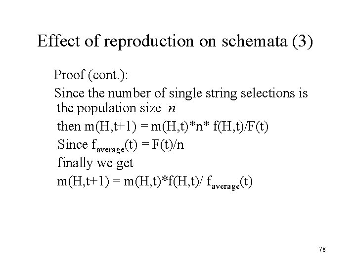
Effect of reproduction on schemata (3) Proof (cont. ): Since the number of single string selections is the population size n then m(H, t+1) = m(H, t)*n* f(H, t)/F(t) Since faverage(t) = F(t)/n finally we get m(H, t+1) = m(H, t)*f(H, t)/ faverage(t) 78

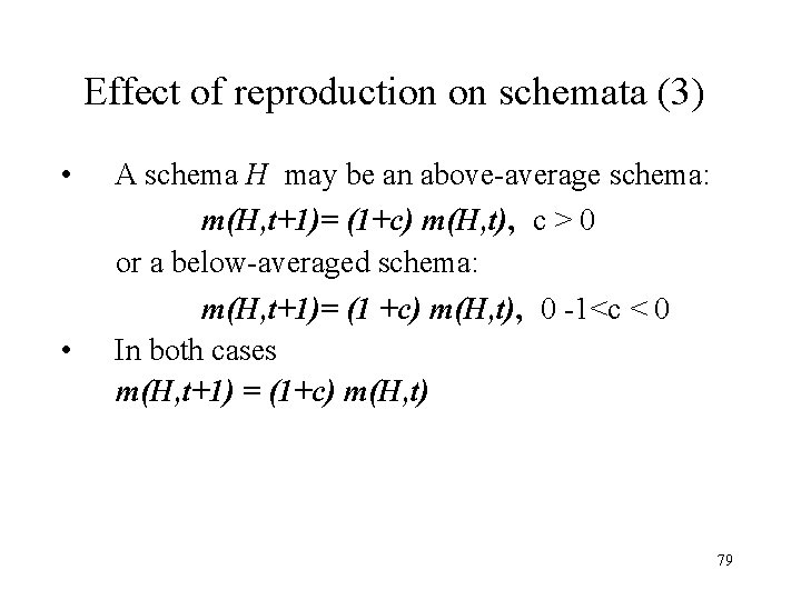
Effect of reproduction on schemata (3) • A schema H may be an above-average schema: m(H, t+1)= (1+c) m(H, t), c > 0 or a below-averaged schema: m(H, t+1)= (1 +c) m(H, t), 0 -1<c < 0 • In both cases m(H, t+1) = (1+c) m(H, t) 79

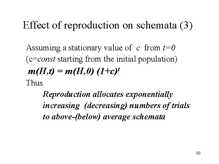
Effect of reproduction on schemata (3) Assuming a stationary value of c from t=0 (c=const starting from the initial population) m(H, t) = m(H, 0) (1+c)t Thus Reproduction allocates exponentially increasing (decreasing) numbers of trials to above-(below) average schemata 80

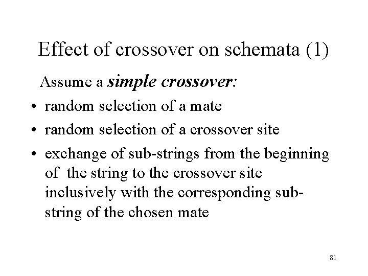
Effect of crossover on schemata (1) Assume a simple crossover: • random selection of a mate • random selection of a crossover site • exchange of sub-strings from the beginning of the string to the crossover site inclusively with the corresponding substring of the chosen mate 81

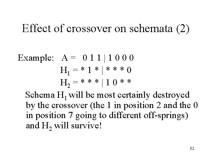
Effect of crossover on schemata (2) Example: A = 0 1 1 | 1 0 0 0 H 1 = * 1 * | * * * 0 H 2 = * * * | 1 0 * * Schema H 1 will be most certainly destroyed by the crossover (the 1 in position 2 and the 0 in position 7 going to different off-springs) and H 2 will survive! 82

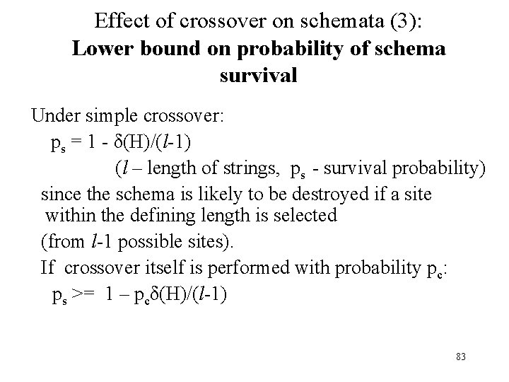
Effect of crossover on schemata (3): Lower bound on probability of schema survival Under simple crossover: ps = 1 - δ(H)/(l-1) (l – length of strings, ps - survival probability) since the schema is likely to be destroyed if a site within the defining length is selected (from l-1 possible sites). If crossover itself is performed with probability pc: ps >= 1 – pcδ(H)/(l-1) 83

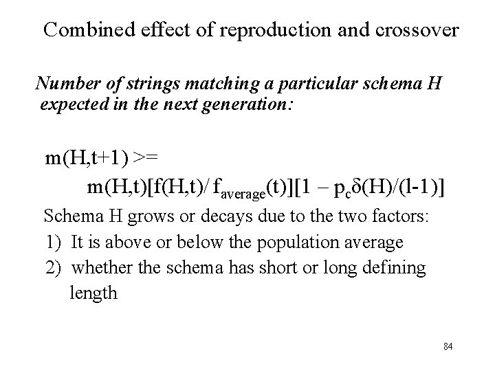
Combined effect of reproduction and crossover Number of strings matching a particular schema H expected in the next generation: m(H, t+1) >= m(H, t)[f(H, t)/ faverage(t)][1 – pcδ(H)/(l-1)] Schema H grows or decays due to the two factors: 1) It is above or below the population average 2) whether the schema has short or long defining length 84

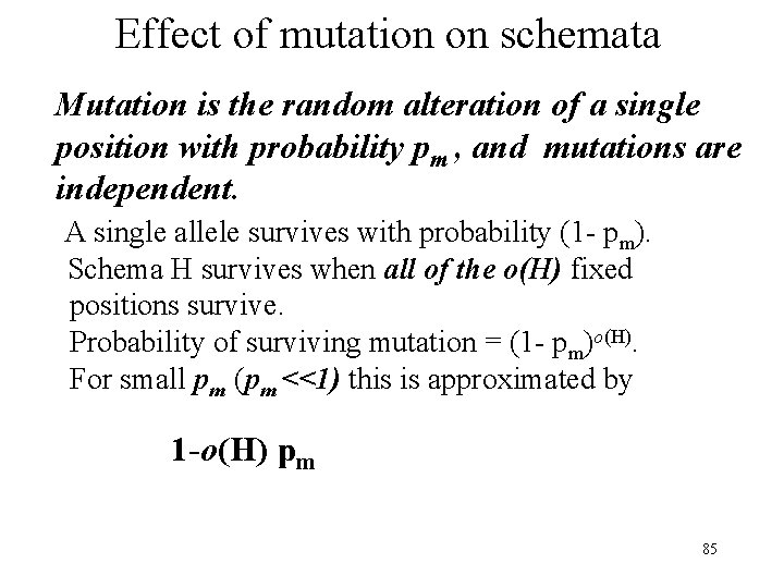
Effect of mutation on schemata Mutation is the random alteration of a single position with probability pm , and mutations are independent. A single allele survives with probability (1 - pm). Schema H survives when all of the o(H) fixed positions survive. Probability of surviving mutation = (1 - pm)o(H). For small pm (pm <<1) this is approximated by 1 -o(H) pm 85

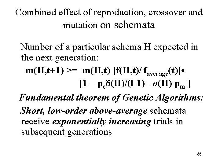
Combined effect of reproduction, crossover and mutation on schemata Number of a particular schema H expected in the next generation: m(H, t+1) >= m(H, t) [f(H, t)/ faverage(t)] • [1 – pcδ(H)/(l-1) - o(H) pm ] Fundamental theorem of Genetic Algorithms: Short, low-order above-average schemata receive exponentially increasing trials in subsequent generations 86

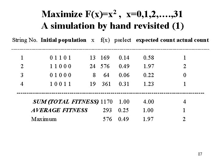
Maximize F(x)=x 2 , x=0, 1, 2, …. , 31 A simulation by hand revisited (1) String No. Initial population x f(x) pselect expected count actual count ------------------------------------------------ 1 0 1 1 0 1 13 169 0. 14 0. 58 1 2 1 1 0 0 0 24 576 0. 49 1. 97 2 3 0 1 0 0 0 8 64 0. 06 0. 22 0 4 1 0 0 1 1 19 361 0. 31 1. 23 1 ----------------------------------------------SUM (TOTAL FITNESS) 1170 1. 00 4. 00 4 AVERAGE FITNESS 293 0. 25 1. 00 1 Maximum 576 0. 49 1. 97 2 87

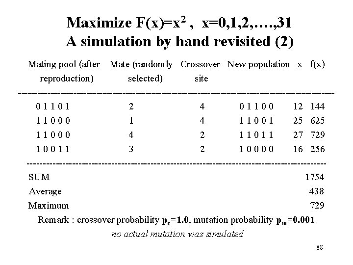
Maximize F(x)=x 2 , x=0, 1, 2, …. , 31 A simulation by hand revisited (2) Mating pool (after Mate (randomly Crossover New population x f(x) reproduction) selected) site ------------------------------------------------ 0 1 1 0 1 2 4 0 1 1 0 0 12 144 1 1 0 0 0 1 4 1 1 0 0 1 25 625 1 1 0 0 0 4 2 1 1 0 1 1 27 729 1 0 0 1 1 3 2 1 0 0 16 256 ----------------------------------------------SUM 1754 Average 438 Maximum 729 Remark : crossover probability pc=1. 0, mutation probability pm=0. 001 no actual mutation was simulated 88

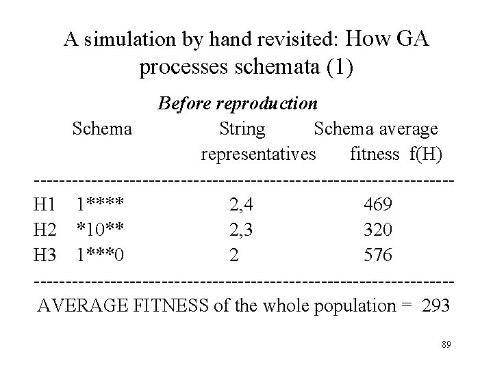
A simulation by hand revisited: How GA processes schemata (1) Before reproduction Schema String Schema average representatives fitness f(H) ---------------------------------H 1 1**** 2, 4 469 H 2 *10** 2, 3 320 H 3 1***0 2 576 --------------------------------- AVERAGE FITNESS of the whole population = 293 89

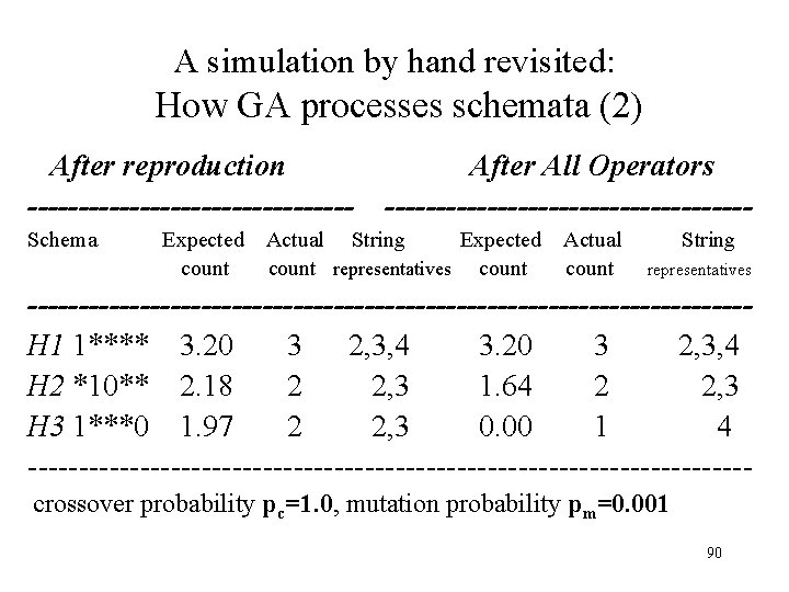
A simulation by hand revisited: How GA processes schemata (2) After reproduction ---------------- After All Operators ------------------ Schema Expected Actual String Expected Actual String count representatives count representatives -----------------------------------H 1 1**** 3. 20 3 2, 3, 4 3. 20 3 2, 3, 4 H 2 *10** 2. 18 2 2, 3 1. 64 2 2, 3 H 3 1***0 1. 97 2 2, 3 0. 00 1 4 ----------------------------------- crossover probability pc=1. 0, mutation probability pm=0. 001 90

How many schemata are processed usefully? (1) • A single string contains 2 l schemata (actual value or * (don’t care) in each of l positions). • A string population of size n and length l contains from 2 l to n. 2 l schemata. • How much of them are processed usefully (that is, with high survival rate)? 91

How many schemata are processed usefully? (2) • Holland’s estimate: at least O(n 3) effective schemata are processed ! • Even though each generation we perform computation proportional to the size of population n, a GA processes something like n 3 schemata. • “Implicit parallelism” 92

Building Block Hypothesis • Short, low-order, and highly fit schemata are called building blocks. • A genetic algorithm seeks near-optimal performance by juxtaposition of building blocks. This means that the building blocks are sampled, recombined and re-sampled to form strings of potentially higher fitness. 93

Coding (1) Principle of meaningful building blocks: Use a coding that short, low-order schemata are relevant to the underlying problem. Principle of minimal alphabets: Select a smallest alphabet that permits a natural representation of the problem. 94

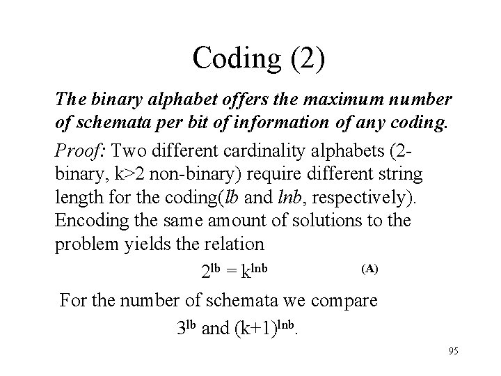
Coding (2) The binary alphabet offers the maximum number of schemata per bit of information of any coding. Proof: Two different cardinality alphabets (2 - binary, k>2 non-binary) require different string length for the coding(lb and lnb, respectively). Encoding the same amount of solutions to the problem yields the relation 2 lb = klnb (A) For the number of schemata we compare 3 lb and (k+1)lnb. 95

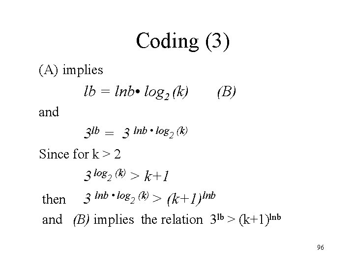
Coding (3) (A) implies lb = lnb • log 2 (k) and (B) 3 lb = 3 lnb • log 2 (k) Since for k > 2 3 log 2 (k) > k+1 then 3 lnb • log 2 (k) > (k+1)lnb and (B) implies the relation 3 lb > (k+1)lnb 96

Part V Traveling Salesman • Problem formulation • Encoding the solution • Genetic operators 97

The traveling salesman problem (TSP) (1) • Given a finite number of "cities" along with the cost of travel between each pair of them, find the cheapest way of visiting all the cities and returning to your starting point. • Blind version of the problem is that where the distances between points are unknown in advance. Such a situation would arise, for example, you might be trying to find the fastest route through the Internet, not knowing how many "hops" exist between nodes. 98

The traveling salesman problem (TSP) (2) • NP-hard. • The number of cities may be quite significant in applications: e. g. , in VLSI fabrication more than 1 million cities was reported already in 1987. • Solution of TSP by GAs: Extremely easy evaluation (fitness) function: for any potential solution (a permutation of cities) the table of distances provides the total length of the tour. 99

The traveling salesman problem (TSP) (3) The difficulty in the TSP using a GA is encoding the solutions. The binary representation is not well suited for the TSP. Three major vector representations exist: 1) Adjacency representation 2) Ordinal representation 3) Path representation In all three representations, a tour is described as a list of cities. Each representation has its own genetic operators. 100

TSP: Adjacency representation (1) The city J is listed in the position I if and only if the tour leads from city I to city J. E. g. the vector (2 4 8 3 9 7 1 5 6) represents the following tour: 1 -2 -4 -3 -8 -5 -9 -6 -7. Each list has only one adjacency representation but some adjacency lists can represents illegal lists: (2 4 8 1 9 3 5 7 6) yields the tour 1 -2 -4 -1 (a premature cycle). The adjacency representation does not support the classical crossover! 101

TSP: Adjacency representation (2) § Alternate-edges crossover : the operator extends the tour by choosing edges from alternating parents. If the new edge causes a cycle, the operator selects instead a random edge from the remaining edges which does not introduce a cycle. § Example: the first off-spring from parents p 1 = (2 3 8 7 9 4 1 5 6) and p 2 = (7 5 1 6 9 2 8 4 3) might be (2 5 8 7 9 1 6 4 3) where the crossover started from the edge (1, 2) from p 1. (The only random edge here is (7, 6) instead of (7, 8) which would cause a premature cycle). 102

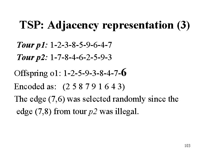
TSP: Adjacency representation (3) Tour p 1: 1 -2 -3 -8 -5 -9 -6 -4 -7 Tour p 2: 1 -7 -8 -4 -6 -2 -5 -9 -3 Offspring o 1: 1 -2 -5 -9 -3 -8 -4 -7 -6 Encoded as: (2 5 8 7 9 1 6 4 3) The edge (7, 6) was selected randomly since the edge (7, 8) from tour p 2 was illegal. 103

TSP: Adjacency representation (4) § Sub-tour-chunks crossover: the operator constructs an offspring by choosing a random length sub-tour from one of the parents, then choosing a random length sub-tour from another etc. Again, if the new edge introduces a cycle into the current (still partial) tour, the operator selects instead a random edge from the remaining edges which does not introduce a cycle. 104

TSP: Adjacency representation (5) Heuristic crossover (A greedy algorithm) builds the tour by choosing a random city as a starting point for the offspring’s tour. Then the operator compares the two edges (from both parents) which leave the city, and a shorter edge is chosen. The city on the other end of the chosen city serves then as a starting point etc. Again, if a new edge introduces a cycle into the partial tour, the operator selects instead a random edge from the remaining edges which does not introduce a cycle. 105

TSP: Adjacency representation (6) Modified heuristic crossover consists of the following two modifications: 1) if the shorter edge (taken from a parent) introduces a cycle in the offspring tour, try the other (longer) edge. If the longer edge is illegal (introduces a cycle) then: 2) select the shortest edge from the pool of q randomly selected legal edges (q is a parameter of the method). A disadvantage of heuristic crossover: undesirable crossings of edges. 106

TSP: Adjacency representation (7) Fine tuning of the heuristic crossover operator: 1) Random selection of two edges (i, j) and (k, m) in the tour. 2) The check if dist(i, j) + dist (k, m) > dist(i, m) + dist(k, j) ? where dist(a, b) is a given distance between cities a and b. 3) If yes, the edges (i, j) and (k, m) are replaced by edges (i, m) and (k, j). 107

TSP: Adjacency representation (8) An advantage of the adjacency representation: Schemata correspond to natural building blocks (edges). For example, the schema (* * * 3 * 7 * * *) represents the set of all tours with edges (4, 3) and (6, 7). The main disadvantage: Relatively poor results for all operators: the alternating-edges crossover often disrupts good tours, the sub-tour-chunks crossover possesses a lower disruption rate, and heuristic crossover is less blind than the previous two since it takes into account the actual lengths but its performance is not outstanding. 108

TSP: Ordinal representation (1) Reference point: a some ordered list of cities C, e. g. simply C = (1 2 3 4 5 6 7 8 9). A tour 1 -2 -4 -3 -8 -5 -9 -6 -7 is then represented as a list l of references, l = (1 1 2 1 4 1 3 1 1). Interpretation of l: Take the first number on l: (1). Then take the first city from the list C (number 1) as the first city of the tour and remove it from C. The next number on l is also (1) so take the first number from the current list C (number 2) as the next city of the tour and remove it from the list C. 109

TSP: Ordinal representation (2) Now the partial tour is 1 -2. Continue the interpretation of l: The next number on the list l is (2). Then take the second city from the current list C (the number 4) as the next city of the tour and remove it from the list C. The partial tour is now 1 -2 -4. The next number on the list l is (1). Then take the first city from the current list C (the number 3) as the next city of the tour and remove it from the list C. The partial tour is now 1 -2 -4 -3 etc. 110

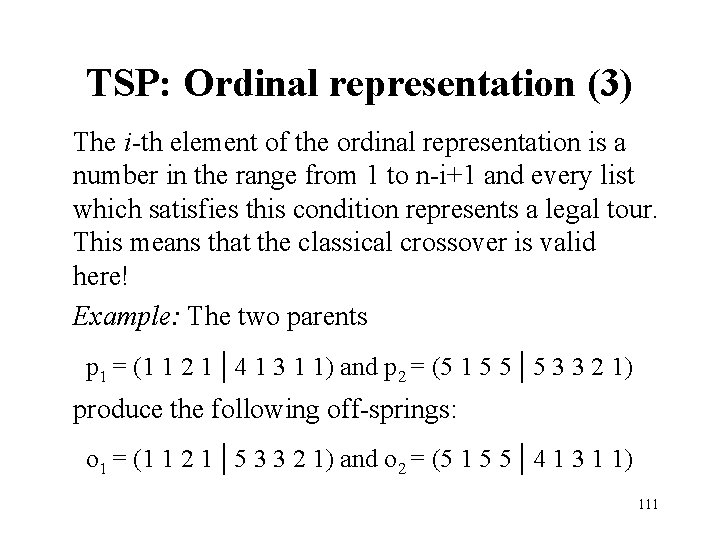
TSP: Ordinal representation (3) The i-th element of the ordinal representation is a number in the range from 1 to n-i+1 and every list which satisfies this condition represents a legal tour. This means that the classical crossover is valid here! Example: The two parents p 1 = (1 1 2 1 | 4 1 3 1 1) and p 2 = (5 1 5 5 | 5 3 3 2 1) produce the following off-springs: o 1 = (1 1 2 1 | 5 3 3 2 1) and o 2 = (5 1 5 5 | 4 1 3 1 1) 111

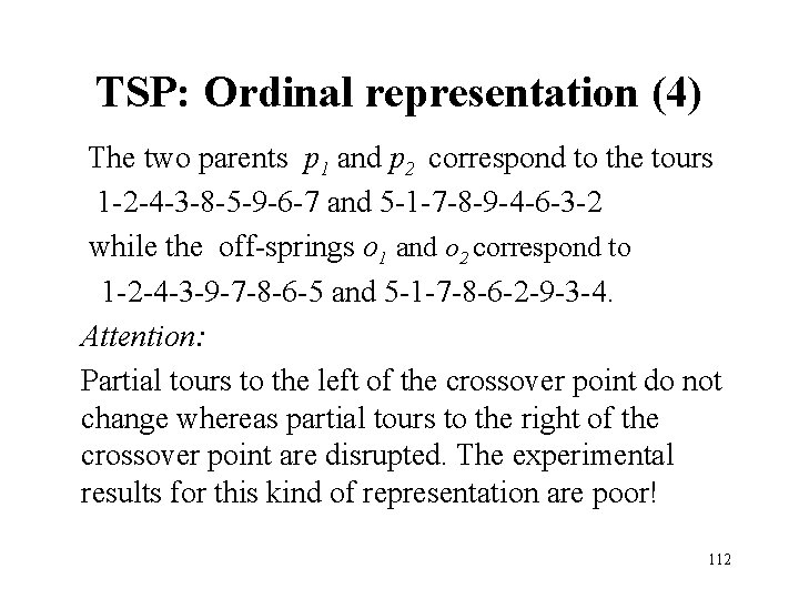
TSP: Ordinal representation (4) The two parents p 1 and p 2 correspond to the tours 1 -2 -4 -3 -8 -5 -9 -6 -7 and 5 -1 -7 -8 -9 -4 -6 -3 -2 while the off-springs o 1 and o 2 correspond to 1 -2 -4 -3 -9 -7 -8 -6 -5 and 5 -1 -7 -8 -6 -2 -9 -3 -4. Attention: Partial tours to the left of the crossover point do not change whereas partial tours to the right of the crossover point are disrupted. The experimental results for this kind of representation are poor! 112

TSP: Path representation (1) The most natural representation of a tour. A tour 5 -1 -7 -8 -9 -4 -6 -2 -3 is represented simply as (5 1 7 8 9 4 6 2 3). It does not support the classical crossover. Three new crossovers for the path representation: Ø PMX: The partially-matched crossover Ø OX: The ordered crossover Ø CX: The cyclic crossover 113

TSP: Path representation (2) PMX: The partially-matched crossover An offspring is built by choosing a subsequence of a tour from one parent and preserving the order and position of as many cities as possible from the other parent. A subsequence of a tour is selected by choosing two random cut points which serve boundaries for swapping operations. E. g. , in the case of two parents p 1 = (1 2 3 | 4 5 6 7 | 8 9) and p 2 = (4 5 2 | 1 8 7 6 | 9 3) offspring is produced in the following way: 114

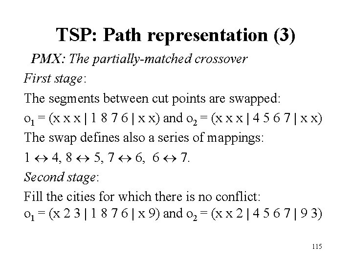
TSP: Path representation (3) PMX: The partially-matched crossover First stage: The segments between cut points are swapped: o 1 = (x x x | 1 8 7 6 | x x) and o 2 = (x x x | 4 5 6 7 | x x) The swap defines also a series of mappings: 1 4, 8 5, 7 6, 6 7. Second stage: Fill the cities for which there is no conflict: o 1 = (x 2 3 | 1 8 7 6 | x 9) and o 2 = (x x 2 | 4 5 6 7 | 9 3) 115

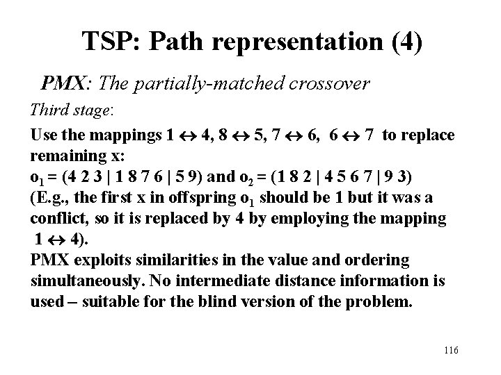
TSP: Path representation (4) PMX: The partially-matched crossover Third stage: Use the mappings 1 4, 8 5, 7 6, 6 7 to replace remaining x: o 1 = (4 2 3 | 1 8 7 6 | 5 9) and o 2 = (1 8 2 | 4 5 6 7 | 9 3) (E. g. , the first x in offspring o 1 should be 1 but it was a conflict, so it is replaced by 4 by employing the mapping 1 4). PMX exploits similarities in the value and ordering simultaneously. No intermediate distance information is used – suitable for the blind version of the problem. 116

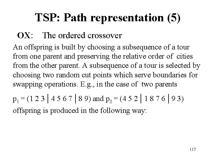
TSP: Path representation (5) OX: The ordered crossover An offspring is built by choosing a subsequence of a tour from one parent and preserving the relative order of cities from the other parent. A subsequence of a tour is selected by choosing two random cut points which serve boundaries for swapping operations. E. g. , in the case of two parents p 1 = (1 2 3 | 4 5 6 7 | 8 9) and p 2 = (4 5 2 | 1 8 7 6 | 9 3) offspring is produced in the following way: 117

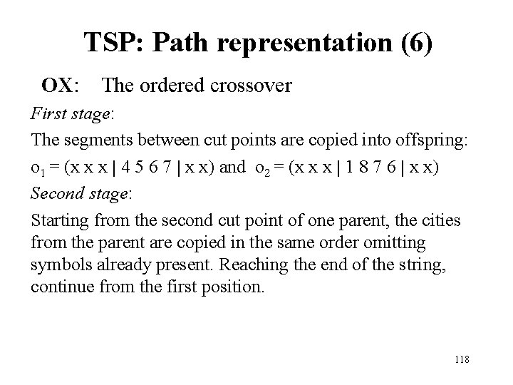
TSP: Path representation (6) OX: The ordered crossover First stage: The segments between cut points are copied into offspring: o 1 = (x x x | 4 5 6 7 | x x) and o 2 = (x x x | 1 8 7 6 | x x) Second stage: Starting from the second cut point of one parent, the cities from the parent are copied in the same order omitting symbols already present. Reaching the end of the string, continue from the first position. 118

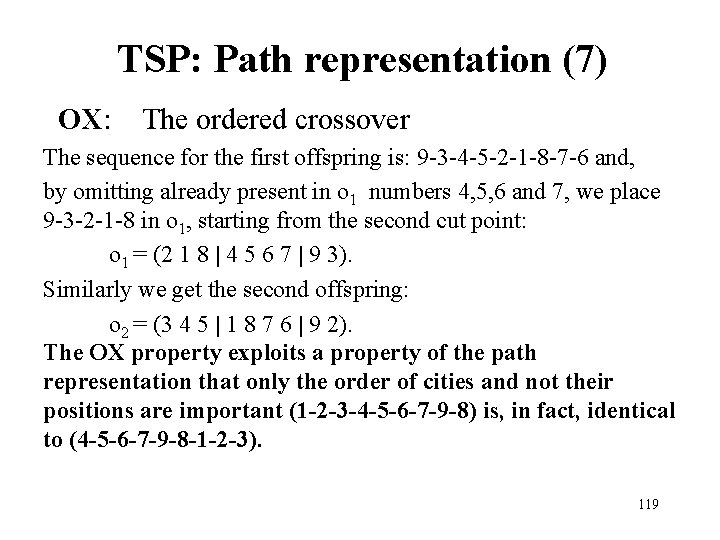
TSP: Path representation (7) OX: The ordered crossover The sequence for the first offspring is: 9 -3 -4 -5 -2 -1 -8 -7 -6 and, by omitting already present in o 1 numbers 4, 5, 6 and 7, we place 9 -3 -2 -1 -8 in o 1, starting from the second cut point: o 1 = (2 1 8 | 4 5 6 7 | 9 3). Similarly we get the second offspring: o 2 = (3 4 5 | 1 8 7 6 | 9 2). The OX property exploits a property of the path representation that only the order of cities and not their positions are important (1 -2 -3 -4 -5 -6 -7 -9 -8) is, in fact, identical to (4 -5 -6 -7 -9 -8 -1 -2 -3). 119

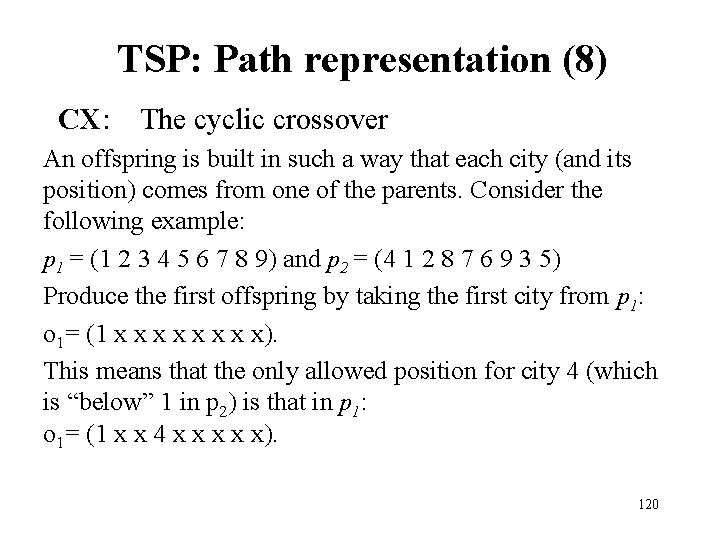
TSP: Path representation (8) CX: The cyclic crossover An offspring is built in such a way that each city (and its position) comes from one of the parents. Consider the following example: p 1 = (1 2 3 4 5 6 7 8 9) and p 2 = (4 1 2 8 7 6 9 3 5) Produce the first offspring by taking the first city from p 1: o 1= (1 x x x x). This means that the only allowed position for city 4 (which is “below” 1 in p 2) is that in p 1: o 1= (1 x x 4 x x x). 120

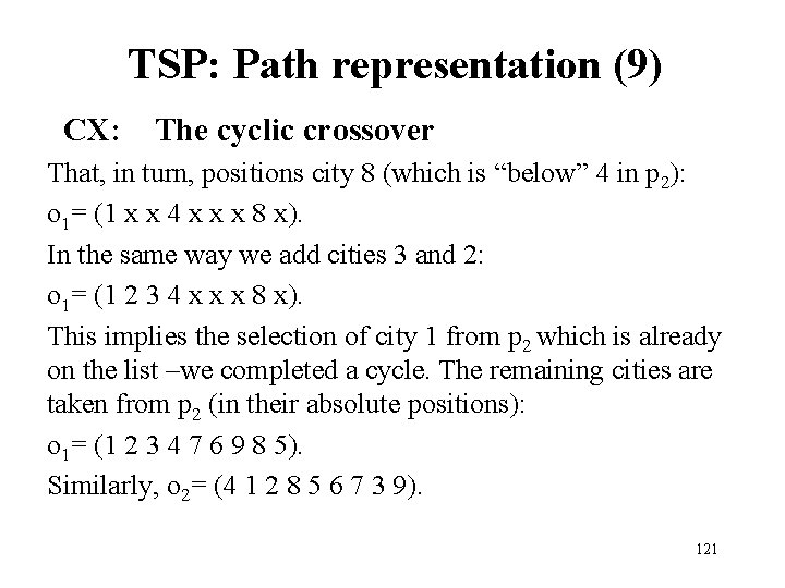
TSP: Path representation (9) CX: The cyclic crossover That, in turn, positions city 8 (which is “below” 4 in p 2): o 1= (1 x x 4 x x x 8 x). In the same way we add cities 3 and 2: o 1= (1 2 3 4 x x x 8 x). This implies the selection of city 1 from p 2 which is already on the list –we completed a cycle. The remaining cities are taken from p 2 (in their absolute positions): o 1= (1 2 3 4 7 6 9 8 5). Similarly, o 2= (4 1 2 8 5 6 7 3 9). 121

Part VI Prisoner’s dilemma • Problem formulation • Coding • Conclusions 122

The iterated prisoner’s dilemma (1) • This is an example how a GA can teach us a game strategy. • The game: two prisoners are held in separate cells, and they are unable to communicate. Each prisoner is asked (independently) to defect and betray the other. If only one prisoner defects, he is rewarded and the other is punished. If both defect, both remain imprisoned and tortured. If neither defects, both receive moderate rewards. • Thus, a selfish detection yields a higher payoff than cooperation (no matter what the other does), but if both defect, both do worse than if both cooperated. • The dilemma is to decide whether to defect or cooperate with other prisoner. 123

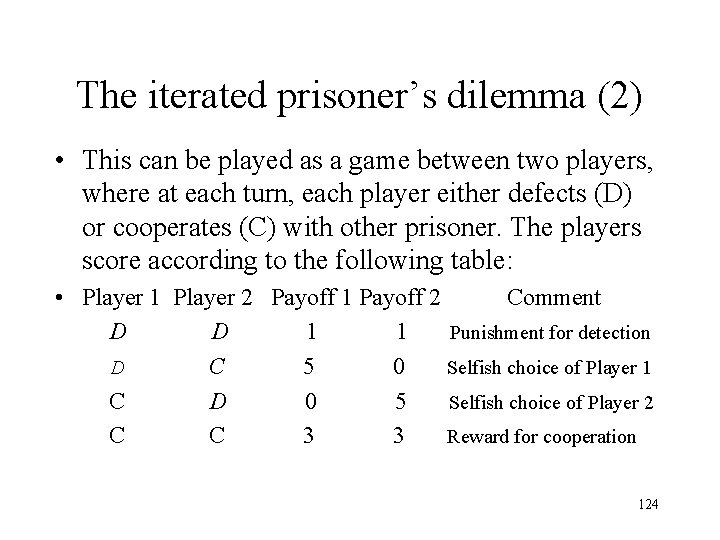
The iterated prisoner’s dilemma (2) • This can be played as a game between two players, where at each turn, each player either defects (D) or cooperates (C) with other prisoner. The players score according to the following table: • Player 1 Player 2 Payoff 1 Payoff 2 Comment D D 1 1 Punishment for detection D C 5 0 Selfish choice of Player 1 C D 0 5 Selfish choice of Player 2 C 3 3 Reward for cooperation 124

The iterated prisoner’s dilemma (3) • GA approach: to maintain a population of players, each of which has a particular strategy. At each step, players play games and score. Some of the players are selected for the next generation, and some of them mate. The new player created has a strategy constructed by crossover of the strategies of the parents. Some mutation is also allowed. • Solutions: deterministic strategies using the results of the three previous moves (64 histories) to make a choice. 125

The iterated prisoner’s dilemma (4) § Each bit (or C or D) in a strategy corresponds to one of 64 possible histories. A move is described by a pair (AB), where A denotes the player’s move (C or D) and B stands for the other player’s move (C or D). § 64 possible histories range from (CC)(CC) to (DD)(DD). Additional 6 bits are needed to code three previous (hypothetical) moves in the beginning of the game. 126

The iterated prisoner’s dilemma (5): Axelrod’s GA • Choice of initial population by assigning a random string of 70 bits. • Each player plays the game with other players using the strategy defined by his chromosome. His score is its average over all the games he plays. • Selection: a player with average score is given one mating, a player with one standard deviation above the average is given 2 matings, and a player with one standard deviation below the average is given no matings. • Random mating with two off-springs per mating. Crossover and mutation determine the strategy of each offspring. 127

The iterated prisoner’s dilemma (6): Axelrod’s GA, Experimental Behavioral Patterns • Don’t rock the boat: continue cooperate after three mutual cooperations: C after (CC)(CC). • Be provokable: defect when other player defects out of the blue: D after (CC)(CD). • Accept an apology: continue to cooperate after cooperation has been restored: C after (CD)(DC)(CC). • Forget: cooperate when mutual cooperation has been restored after an exploitation: C after (DC)(CC). • Defect after three mutual defections: D after (DD)(DD). Remark: in a pair (AB) A is the player’s move and B is the other player’s move. 128

The iterated prisoner’s dilemma (6): Axelrod’s GA, Experimental Behavioral Patterns • The developed effective strategies are better than previously known and successful “tit for tat” strategy (first cooperate and then do whatever your opponent did on the previous move). • It appeared that it is better not “to be nice” and to defect on the first move (and sometimes even on the second) and use the choices of the other player to discriminate what should be done next! 129

Part VII Advanced Genetic Coding • Fitness function • Multi-parameter coding • Floating-point coding 130

Objective function in non-negative fitness form • A fitness function must be nonnegative. • Possible mappings of the objective function to a fitness function form: 1) For a minimization problem (transformed to maximization problem): f(x) = Cmax – g(x) when 0 < Cmax– g(x), =0 otherwise, 2) For a maximization problem: f(x) = -Cmin + g(x) when 0 < -Cmin+ g(x), =0 otherwise. Cmax and Cmin are estimated lower and upper bound of the objective function g(x): Cmax > g(x), Cmin < g(x). 131

Fitness scaling (1) Scaling in GAs means a transformation of the objective function which does not change the hierarchy of solutions in terms of their fitness. Scaling is useful in several instances: At the start of a GA run, where several “very good” representatives may dominate the selection process. In this case objective function values must be scaled down in order to prevent takeover of population by these “super-strings” (which leads to a premature convergence). 132

Fitness scaling (2) On a later stage, the population average fitness may be close to the population best fitness which promotes mediocre members. In this case the objective function values must be scaled up in order to continue to reward the best performers. 3 major scaling methods: v Linear scaling v Sigma truncation v Power law scaling 133

Fitness scaling (3) Linear scaling: fs = af + b Usually a and b are chosen in order to ensure that 1) average fitness does not change 2) maximum scaled fitness is a specified multiple of the average fitness. This allows 1) average population members receive 1 offspring on average 2) the best receive the specified number of copies. Problem: negative scaled fitness! 134

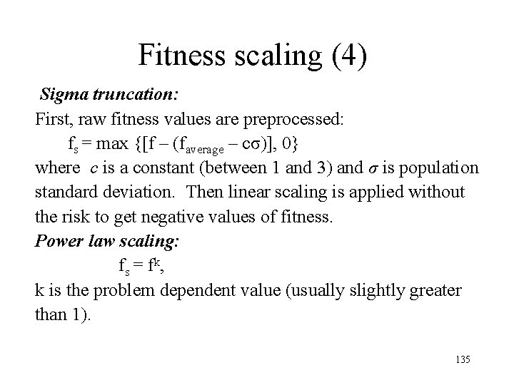
Fitness scaling (4) Sigma truncation: First, raw fitness values are preprocessed: fs = max {[f – (faverage – cσ)], 0} where c is a constant (between 1 and 3) and σ is population standard deviation. Then linear scaling is applied without the risk to get negative values of fitness. Power law scaling: fs = fk, k is the problem dependent value (usually slightly greater than 1). 135

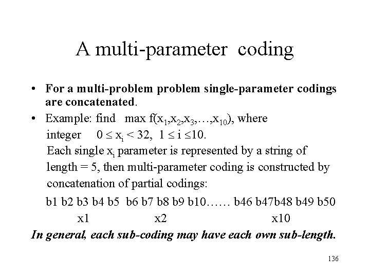
A multi-parameter coding • For a multi-problem single-parameter codings are concatenated. • Example: find max f(x 1, x 2, x 3, …, x 10), where integer 0 xi < 32, 1 i 10. Each single xi parameter is represented by a string of length = 5, then multi-parameter coding is constructed by concatenation of partial codings: b 1 b 2 b 3 b 4 b 5 b 6 b 7 b 8 b 9 b 10…… b 46 b 47 b 48 b 49 b 50 x 1 x 2 x 10 In general, each sub-coding may have each own sub-length. 136

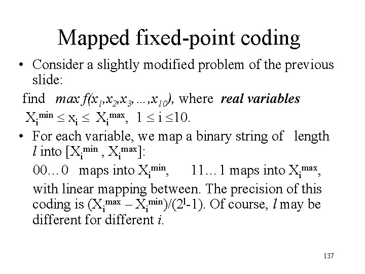
Mapped fixed-point coding • Consider a slightly modified problem of the previous slide: find max f(x 1, x 2, x 3, …, x 10), where real variables Ximin xi Ximax, 1 i 10. • For each variable, we map a binary string of length l into [Ximin , Ximax]: 00… 0 maps into Ximin, 11… 1 maps into Ximax, with linear mapping between. The precision of this coding is (Ximax – Ximin)/(2 l-1). Of course, l may be different for different i. 137

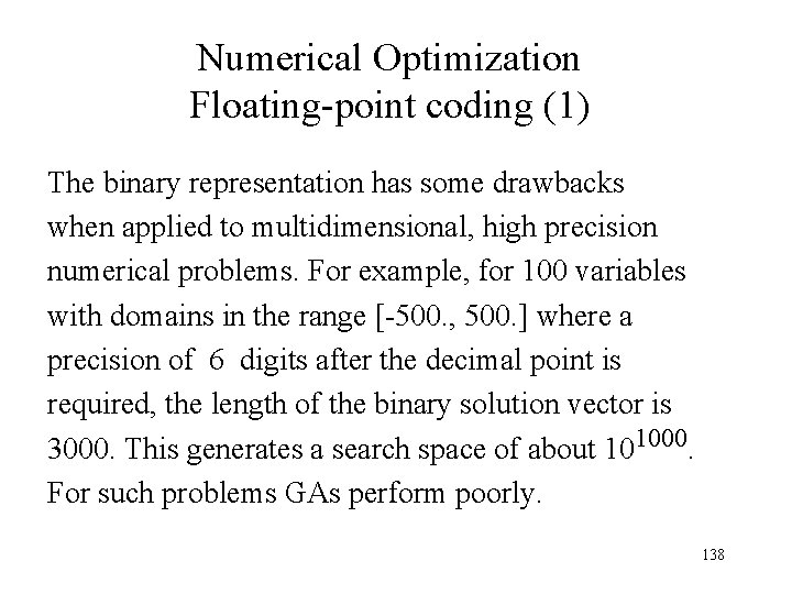
Numerical Optimization Floating-point coding (1) The binary representation has some drawbacks when applied to multidimensional, high precision numerical problems. For example, for 100 variables with domains in the range [-500. , 500. ] where a precision of 6 digits after the decimal point is required, the length of the binary solution vector is 3000. This generates a search space of about 101000. For such problems GAs perform poorly. 138

Numerical Optimization Floating-point coding (2) • With FP coding, each chromosome vector is coded as a vector of floating point numbers, of the same length as the solution vector. FP is a natural coding for continuous solution spaces. • FP coding is able of representation of quite large domains keeping the accuracy of the machine. In binary coding, the extension of accuracy extends the lengths of coded strings and usually slows down the algorithm. • In the framework of FP coding, it is much easier to handle non-trivial constraints. 139

Numerical Optimization Floating-point coding (3) FP Coding: A chromosome (solution) is a vector of floating-point numbers: sv= (v 1, v 2, …. , vn), where each floating point number vk lies in a prescribed range [Lk, Uk], where Lk and Uk are the lower and upper bounds for variable k. FP Selection: Analogous to that of the binary coding 140

Numerical Optimization FP coding: Crossover (1) Crossover: • Single-point crossover: the only permissible split points are between float numbers (v’s) (and not between bits as was the case for the binary coding). • Multipoint crossover: several split points (between float numbers). Both crossover operators are applied as a simple crossover or arithmetical crossover (see the next slide). 141

Numerical Optimization FP coding: Crossover (2) § Simple crossover: Defined in the usual way (the parents swap the corresponding segments of their vectors) § Arithmetical crossover: Defined as a linear combination of two vectors: If sv and sw are crossed, the offspring are: ov=asw + (1 -a)sv and ow=asv + (1 -a)sw , where a is a random value, 0 < a <1. 142

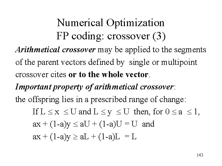
Numerical Optimization FP coding: crossover (3) Arithmetical crossover may be applied to the segments of the parent vectors defined by single or multipoint crossover cites or to the whole vector. Important property of arithmetical crossover: the offspring lies in a prescribed range of change: If L x U and L y U then, for 0 a 1, ax + (1 -a)y a. U + (1 -a)U = U and ax + (1 -a)y a. L + (1 -a)L = L 143

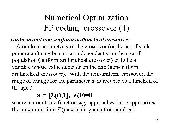
Numerical Optimization FP coding: crossover (4) Uniform and non-uniform arithmetical crossover: A random parameter a of the crossover (or the set of such parameters) may be chosen independently on the age of population (uniform arithmetical crossover) or to be a variable whose value depends on the age (non-uniform arithmetical crossover). With the non-uniform crossover, the range of change for the parameter a is reduced as a function of the age t: a [ (t), 1], (0)=0 where a monotonic function (t) approaches 1 as t approaches the maximum time T (maximum generation number). 144

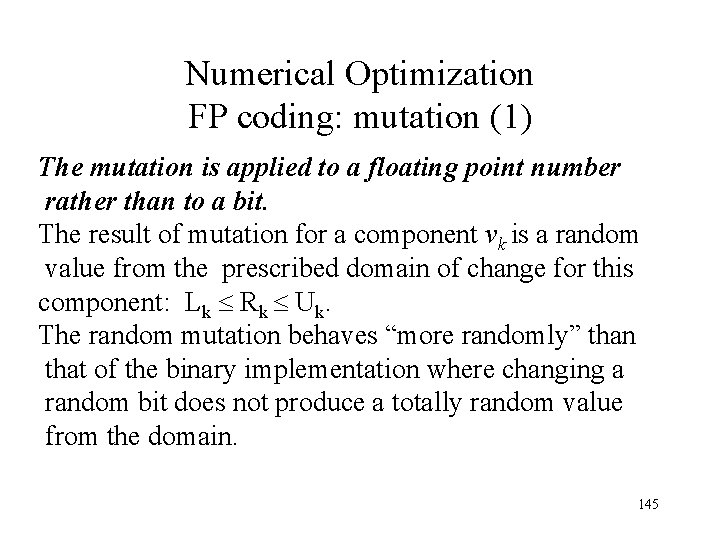
Numerical Optimization FP coding: mutation (1) The mutation is applied to a floating point number rather than to a bit. The result of mutation for a component vk is a random value from the prescribed domain of change for this component: Lk Rk Uk. The random mutation behaves “more randomly” than that of the binary implementation where changing a random bit does not produce a totally random value from the domain. 145

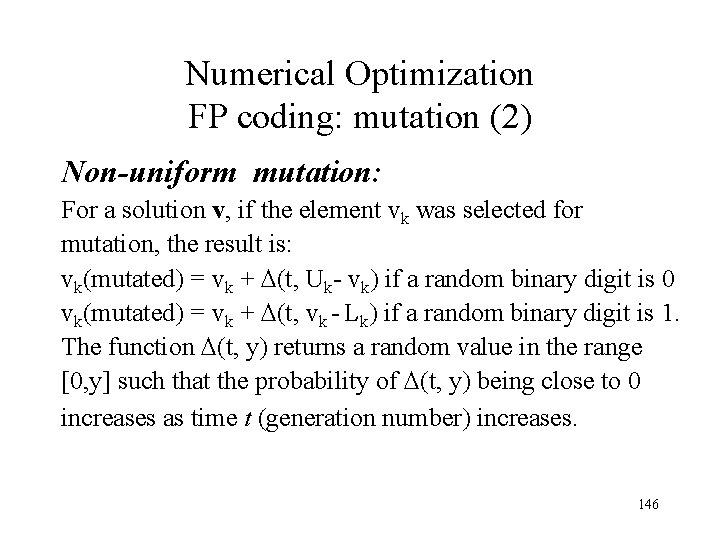
Numerical Optimization FP coding: mutation (2) Non-uniform mutation: For a solution v, if the element vk was selected for mutation, the result is: vk(mutated) = vk + (t, Uk- vk) if a random binary digit is 0 vk(mutated) = vk + (t, vk - Lk) if a random binary digit is 1. The function (t, y) returns a random value in the range [0, y] such that the probability of (t, y) being close to 0 increases as time t (generation number) increases. 146

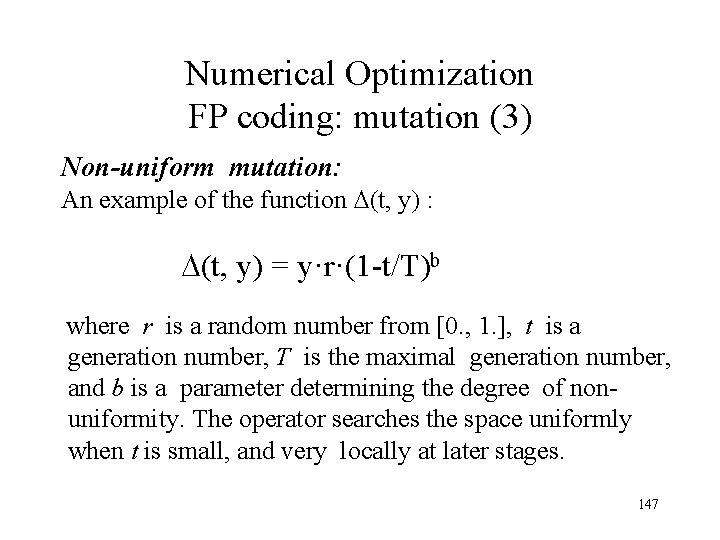
Numerical Optimization FP coding: mutation (3) Non-uniform mutation: An example of the function (t, y) : (t, y) = y·r·(1 -t/T)b where r is a random number from [0. , 1. ], t is a generation number, T is the maximal generation number, and b is a parameter determining the degree of non uniformity. The operator searches the space uniformly when t is small, and very locally at later stages. 147

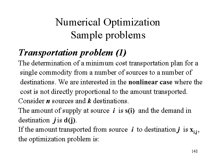
Numerical Optimization Sample problems Transportation problem (1) The determination of a minimum cost transportation plan for a single commodity from a number of sources to a number of destinations. We are interested in the nonlinear case where the cost is not directly proportional to the amount transported. Consider n sources and k destinations. The amount of supply at source i is s(i) and the demand in destination j is d(j). If the amount transported from source i to destination j is xi, j, the optimization problem is: 148

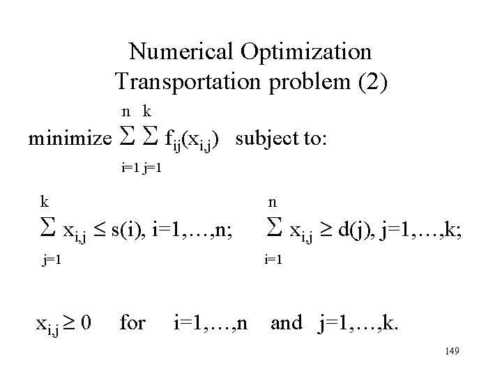
Numerical Optimization Transportation problem (2) n k minimize fij(xi, j) subject to: i=1 j=1 k n xi, j s(i), i=1, …, n; xi, j d(j), j=1, …, k; j=1 i=1 x 0 for i=1, …, n and j=1, …, k. i, j 149

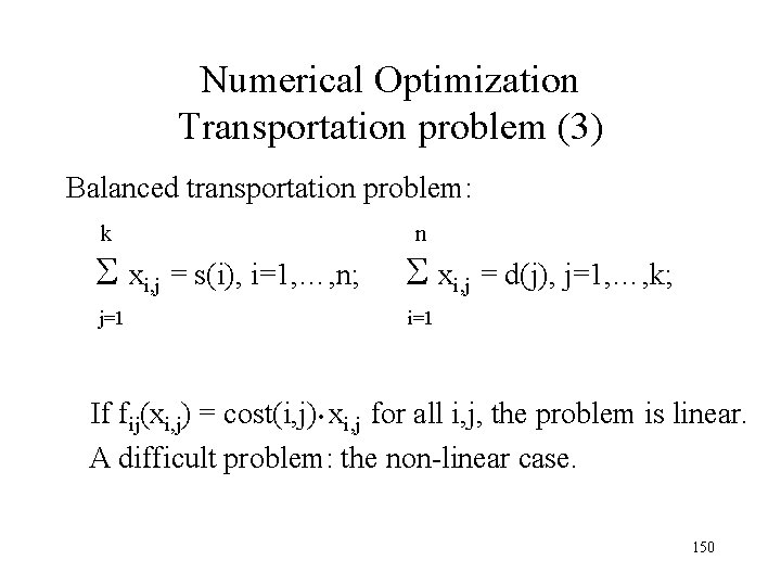
Numerical Optimization Transportation problem (3) Balanced transportation problem: k n xi, j = s(i), i=1, …, n; xi, j = d(j), j=1, …, k; j=1 i=1 If fij(xi, j) = cost(i, j) • xi, j for all i, j, the problem is linear. A difficult problem: the non-linear case. 150

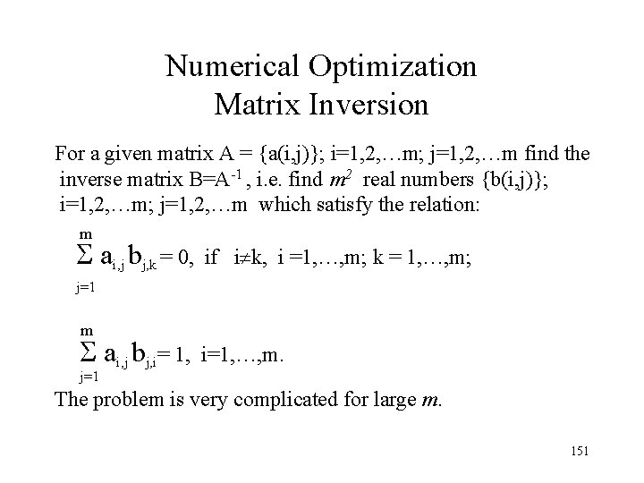
Numerical Optimization Matrix Inversion For a given matrix A = {a(i, j)}; i=1, 2, …m; j=1, 2, …m find the inverse matrix B=A-1 , i. e. find m 2 real numbers {b(i, j)}; i=1, 2, …m; j=1, 2, …m which satisfy the relation: m ai, j bj, k = 0, if i k, i =1, …, m; k = 1, …, m; j=1 m ai, j bj, i= 1, i=1, …, m. j=1 The problem is very complicated for large m. 151

Part VIII Optimization with constraints • Penalty function • Clarifying example • Constraints handling by a new discontinuous method 152

Constraints: Penalty function method (1) • Many practical problems contain constraints. • For highly constrained problem, finding a feasible point is difficult. • The idea: to get some information out of infeasible solutions, degrading their fitness according to the constraint violation. • Thus a constrained problem is transformed to an unconstrained problem. 153

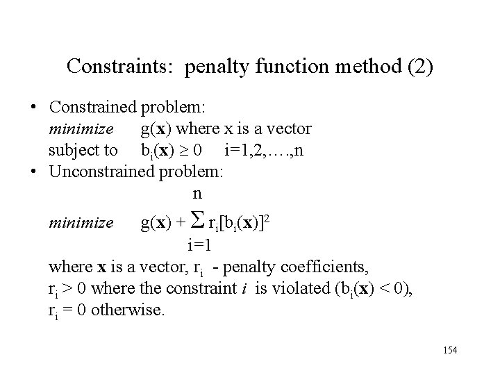
Constraints: penalty function method (2) • Constrained problem: minimize g(x) where x is a vector subject to bi(x) 0 i=1, 2, …. , n • Unconstrained problem: n minimize g(x) + Σ ri[bi(x)]2 i=1 where x is a vector, ri - penalty coefficients, ri > 0 where the constraint i is violated (bi(x) < 0), ri = 0 otherwise. 154

Constraints: penalty function method (3) The construction of penalty functions is a nontrivial and problem-dependent task. It is especially true where the optimum of the unconstrained problem is found inside the infeasible region, and in the challenging case where the optimum of the constrained problem is located on the constraint boundary and this boundary is not known in advance. 155

Penalty method: A clarifying example (1) Find the minimum of the function: F(x, y) = y 2+x 2+y-x+1 in the square [-1. , 1. ]x[-1. , 1] under the constraint g(x, y) = y-x 0 We consider this problem as a model case for a more complicated problem in which the objective function FF(x, y) and the constraint gg(x, y) behave approximately as F and g, but their values are provided by a black box with entries x, y and outputs F(x, y) and g(x, y). 156

Penalty method: A clarifying example (2) In the unconstrained case, the global minimum of the function F(x, y) = y 2+x 2+y-x+1 in the square [-1. , 1. ]x[-1. , 1] is achieved in the point x= 0. 5, y= - 0. 5. Its value is equal to 0. 5. Under the constraint g(x, y) = y-x 0, the minimum is located on the constraint boundary at the point x=0. , y=0. (its value is equal to 1. ) It is easily verified that, at every point (x 0, y 0) located above the line x=y (y 0 > x 0), the value of the objective function F(x, y) is less optimal than that at the point which is the projection of (x 0, y 0) on the line x=y (which has the coordinates x=y = 0. 5(x 0+y 0)). 157

Penalty method: A clarifying example (3) This means that not only that the minimum of the constrained problem minimum lies on the constraint boundary, but, in a sense, the points located in the infeasible region are “more optimal” than those across the boundary. This situation is representative of what frequently happens in “real life” problems. Examples: a budgeting problem with a constraint imposed on the total sum of allocations, or the problem of drag minimization for airfoils with a constraint imposed on the maximum allowed airfoil thickness. 158

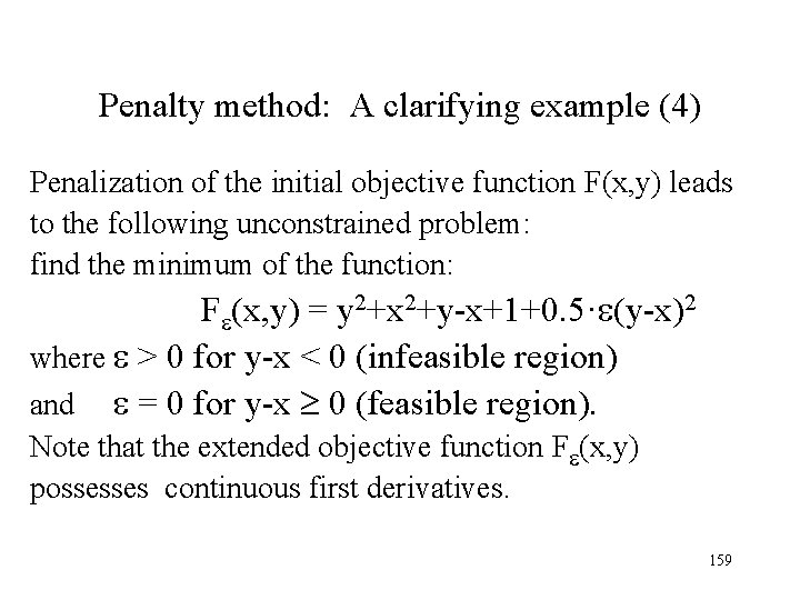
Penalty method: A clarifying example (4) Penalization of the initial objective function F(x, y) leads to the following unconstrained problem: find the minimum of the function: F (x, y) = y 2+x 2+y-x+1+0. 5· (y-x)2 where > 0 for y-x < 0 (infeasible region) and = 0 for y-x 0 (feasible region). Note that the extended objective function F (x, y) possesses continuous first derivatives. 159

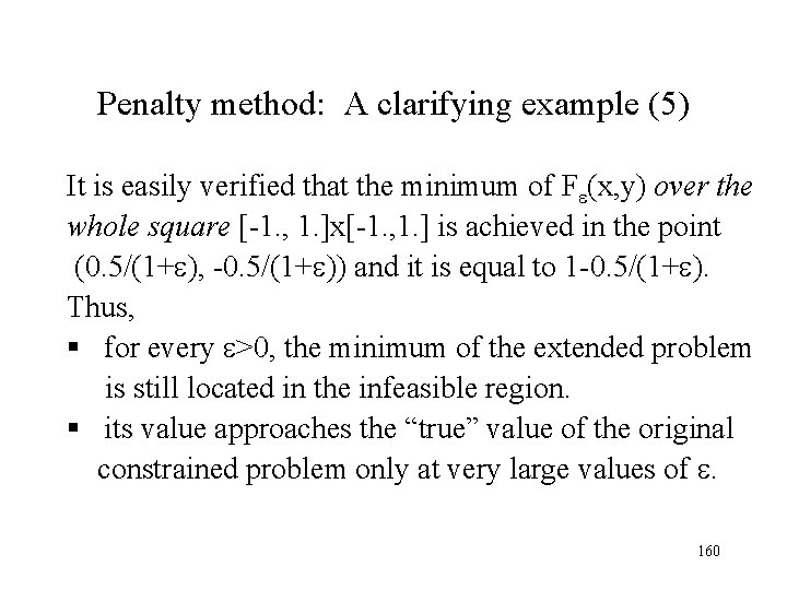
Penalty method: A clarifying example (5) It is easily verified that the minimum of F (x, y) over the whole square [-1. , 1. ]x[-1. , 1. ] is achieved in the point (0. 5/(1+ ), -0. 5/(1+ )) and it is equal to 1 -0. 5/(1+ ). Thus, § for every >0, the minimum of the extended problem is still located in the infeasible region. § its value approaches the “true” value of the original constrained problem only at very large values of . 160

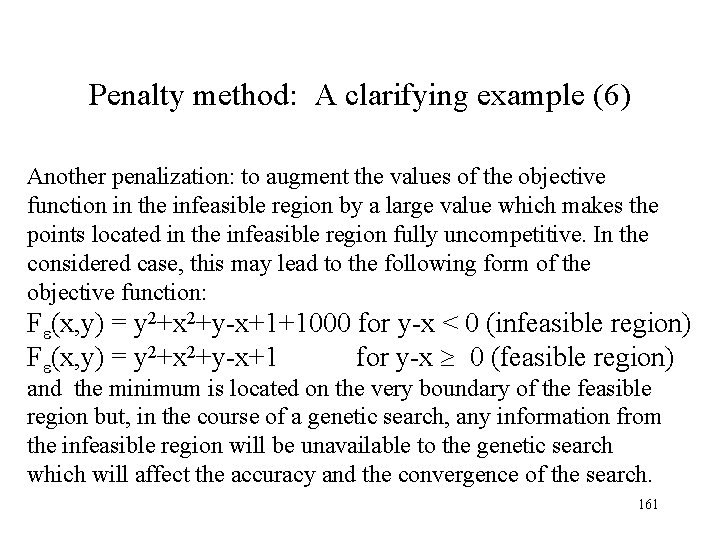
Penalty method: A clarifying example (6) Another penalization: to augment the values of the objective function in the infeasible region by a large value which makes the points located in the infeasible region fully uncompetitive. In the considered case, this may lead to the following form of the objective function: F (x, y) = y 2+x 2+y-x+1+1000 for y-x < 0 (infeasible region) F (x, y) = y 2+x 2+y-x+1 for y-x 0 (feasible region) and the minimum is located on the very boundary of the feasible region but, in the course of a genetic search, any information from the infeasible region will be unavailable to the genetic search which will affect the accuracy and the convergence of the search. 161

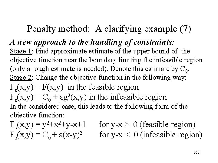
Penalty method: A clarifying example (7) A new approach to the handling of constraints: Stage 1: Find approximate estimate of the upper bound of the objective function near the boundary limiting the infeasible region (only a rough estimate is needed). Denote this estimate by C 0. Stage 2: Change the objective function in the following way: F (x, y) = F(x, y) in the feasible region F (x, y) = C 0 + g 2(x, y) in the infeasible region In the considered case, this leads to the following form of the objective function: F (x, y) = y 2+x 2+y-x+1 for y-x 0 (feasible region) F (x, y) = C 0 + (x-y)2 for y-x < 0 (infeasible region) 162

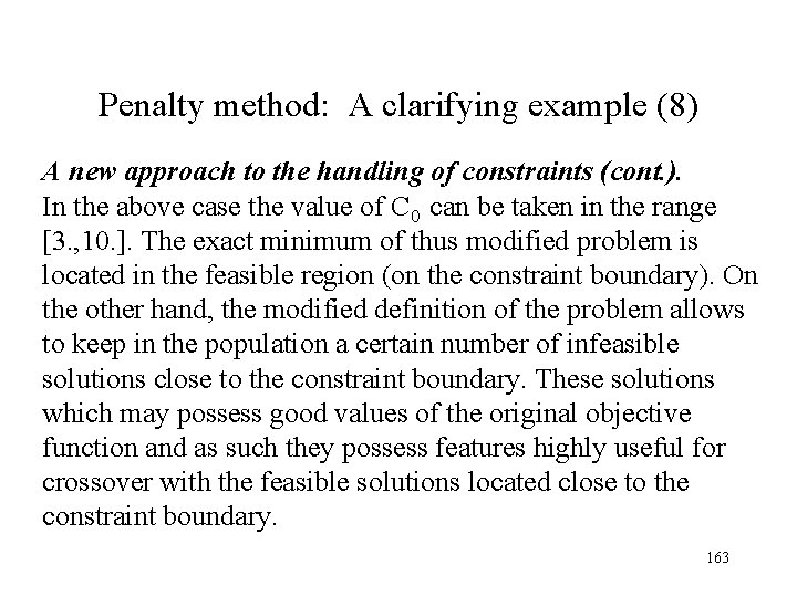
Penalty method: A clarifying example (8) A new approach to the handling of constraints (cont. ). In the above case the value of C 0 can be taken in the range [3. , 10. ]. The exact minimum of thus modified problem is located in the feasible region (on the constraint boundary). On the other hand, the modified definition of the problem allows to keep in the population a certain number of infeasible solutions close to the constraint boundary. These solutions which may possess good values of the original objective function and as such they possess features highly useful for crossover with the feasible solutions located close to the constraint boundary. 163

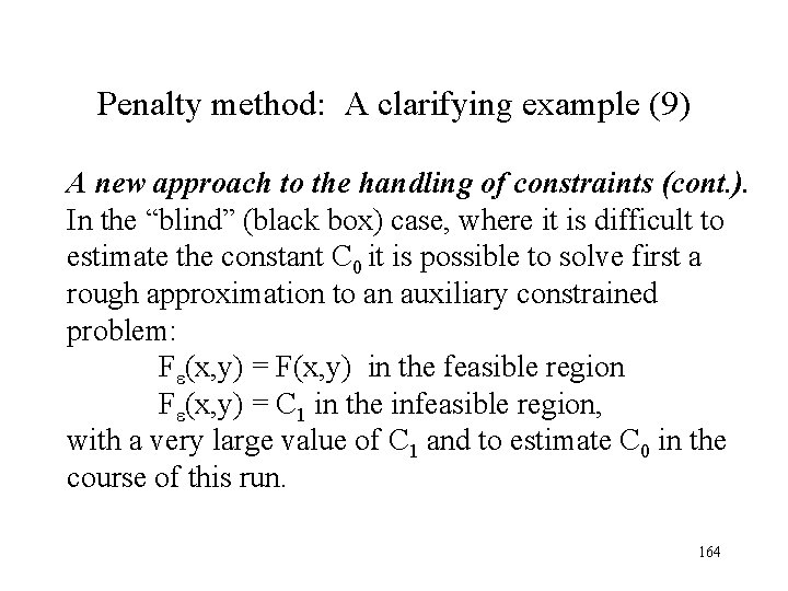
Penalty method: A clarifying example (9) A new approach to the handling of constraints (cont. ). In the “blind” (black box) case, where it is difficult to estimate the constant C 0 it is possible to solve first a rough approximation to an auxiliary constrained problem: F (x, y) = F(x, y) in the feasible region F (x, y) = C 1 in the infeasible region, with a very large value of C 1 and to estimate C 0 in the course of this run. 164

Part IX Advanced topics • • Time-tabling problem Test coverage Multi-objective optimization Hybrid approach 165

Time-tabling problem • Introduction to the Time-tabling Problem • GA Solution for Time-table builder • Hyper-heurestic Approach 166

Time-tabling problem • A variant of the resources allocation problem • Becomes especially difficult in the presence of constraints • Step-by-step approach driven by GAs 167

Time-tabling problem Problem Formulation • A set of events E to be scheduled in time slots • A set of rooms R in which an event can take place (each room has a size) • A set of students S who attend the events (each student attends a number of events) • A set of features F required by events 168

Time-tabling problem Feasible solutions A feasible timetable is one in which all events have been assigned to a timeslot and a room in such a way that the following hard constraints are satisfied: - no student attends more than one event at the same time - the room is big enough to comprise all the students - the room features all the required features - only one event at each room is permitted 169

Time-tabling problem Soft constraints A candidate timetable is penalized for each violation of the following soft constraints: • A student has a class in the last slot of the day • A student has more than two classes (events) in a row • A student has a single class on a day 170

Time-tabling problem GA Solution Time table builder (1) • The algorithm is based on sequential assignment of events • Each event, in each turn, is assigned to a room and then to a timeslot 171

Time-tabling problem GA Solution Time table builder (2) For |E| iterations do 3 steps: (i) choose an unprocessed event e Є E (ii) assign a room r Є R to e (iii) assign the pair <e, r> to a timeslot How to choose an event, room or a time-slot? 172

Time-tabling problem GA Solution Time table builder (2) • Individuals (solutions) for GA represent heuristic rules • Specifically each individual is encoded as a three row matrix (“choose event” row, “assign room” row and “assign timeslot” row), with the number of columns equal to the number of events |E| (equal to the number of assignment iterations) 173

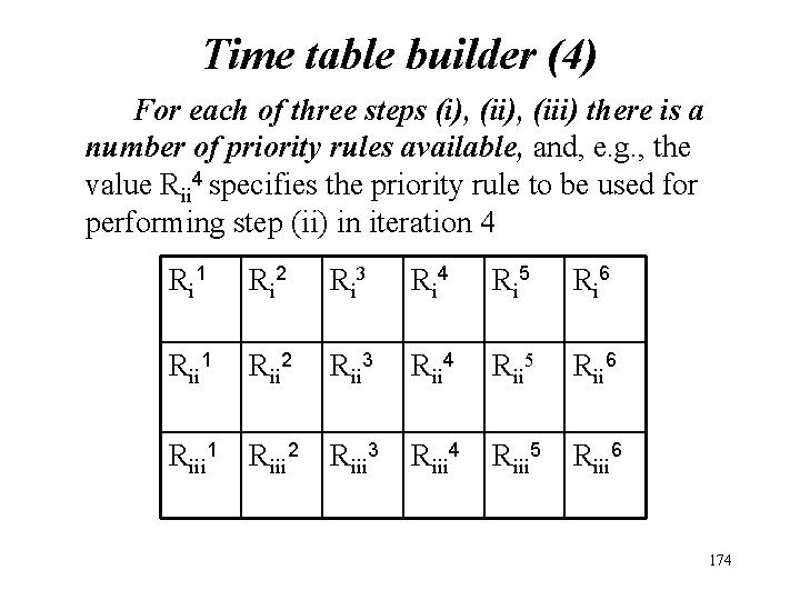
Time table builder (4) For each of three steps (i), (iii) there is a number of priority rules available, and, e. g. , the value Rii 4 specifies the priority rule to be used for performing step (ii) in iteration 4 R i 1 R i 2 R i 3 R i 4 R i 5 R i 6 Rii 1 Rii 2 Rii 3 Rii 4 Rii 5 Rii 6 Riii 1 Riii 2 Riii 3 Riii 4 Riii 5 Riii 6 174

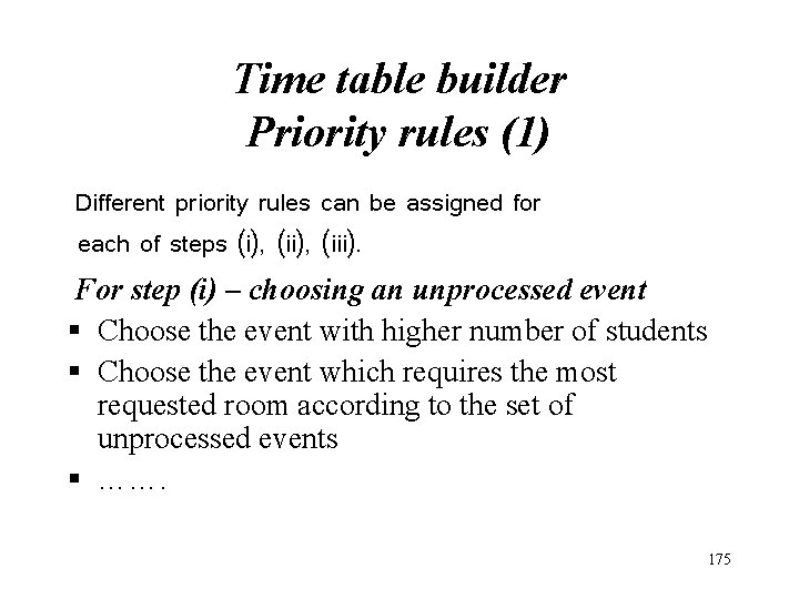
Time table builder Priority rules (1) Different priority rules can be assigned for each of steps (i), (iii). For step (i) – choosing an unprocessed event § Choose the event with higher number of students § Choose the event which requires the most requested room according to the set of unprocessed events § ……. 175

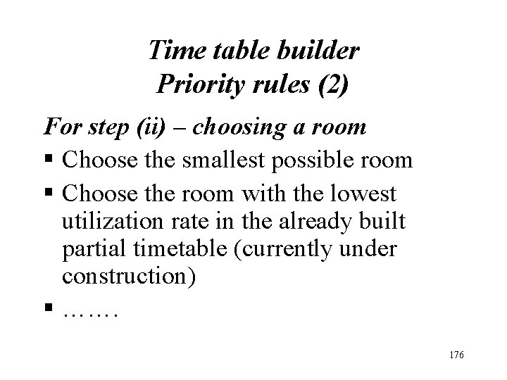
Time table builder Priority rules (2) For step (ii) – choosing a room § Choose the smallest possible room § Choose the room with the lowest utilization rate in the already built partial timetable (currently under construction) § ……. 176

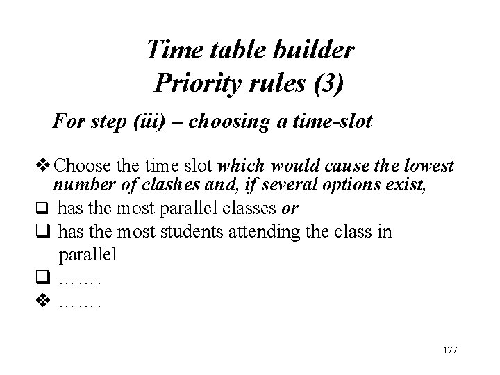
Time table builder Priority rules (3) For step (iii) – choosing a time-slot v Choose the time slot which would cause the lowest number of clashes and, if several options exist, q has the most parallel classes or q has the most students attending the class in parallel q ……. v ……. 177

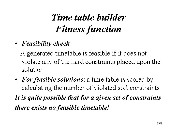
Time table builder Fitness function • Feasibility check A generated timetable is feasible if it does not violate any of the hard constraints placed upon the solution • For feasible solutions: a time table is scored by calculating the number of violated soft constraints It is quite possible that for a given set of constraints there exists no feasible timetable! 178

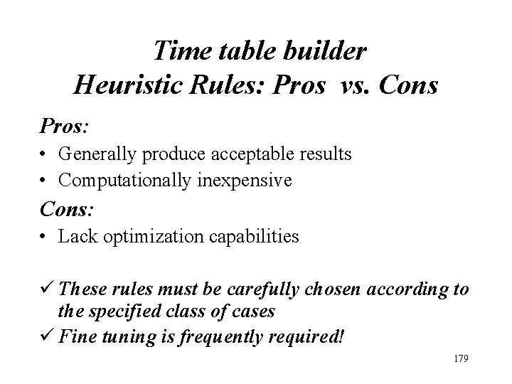
Time table builder Heuristic Rules: Pros vs. Cons Pros: • Generally produce acceptable results • Computationally inexpensive Cons: • Lack optimization capabilities ü These rules must be carefully chosen according to the specified class of cases ü Fine tuning is frequently required! 179

Tame-tabling Problem: Hyper-heuristic Approach (1) • Reference: Rossi-Dorio, Paechter and others The idea: to overcome the weakness of the previous algorithm 1) by introducing changes to the algorithm (see below) and 2) by using much greater variety of heuristic rules 180

Tame-tabling Problem: Hyper-heuristic Approach (2) • Here, an individual comprises two rows representing different (simple) heuristics for use in each of the two steps of the modified builder • Thus an individual represents a two-row matrix with |E| columns 181

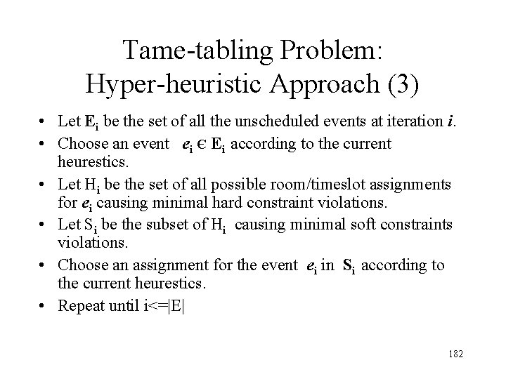
Tame-tabling Problem: Hyper-heuristic Approach (3) • Let Ei be the set of all the unscheduled events at iteration i. • Choose an event ei Є Ei according to the current heurestics. • Let Hi be the set of all possible room/timeslot assignments for ei causing minimal hard constraint violations. • Let Si be the subset of Hi causing minimal soft constraints violations. • Choose an assignment for the event ei in Si according to the current heurestics. • Repeat until i<=|E| 182

Tame-tabling Problem: Hyper-heuristic Approach (4) New algorithm vs. the previous one: 3 major changes: A. A room and a timeslot are chosen in the same construction step vs. two-step procedure (where choice of room was followed by choice of a timeslot) This allows for easier access to the constraint violations of the assignments 183

Tame-tabling Problem: Hyper-heuristic Approach (5) B. Introduction of context into the choice of the pair (room/timeslot): This allows for the choice from the set of “best choices” C. A much larger variety of heuristic rules 184

Tame-tabling Problem: Hyper-heuristic Rules (1) Choosing an event: Ø Maximum number of student clashes with other events Ø Maximum number of students Ø Maximum number of features required by an event Ø Minimum number of available feasible rooms Ø …… Ø Combinations of the above 185

Tame-tabling Problem: Hyper-heuristic Rules (2) Choosing a room and timeslot pair: Ø Smallest possible room Ø Room suitable for minimum events Ø Least used room Ø Latest (or earliest) timeslot of the day Ø Latest or earliest week-day Ø …… Ø Combinations of the above 186

Generating Software Test Data (1) • Automatic software testing by using GAs for test data generation • The goal to verify software quality by finding extreme situations, bottlenecks or faulty behavior • Application to different kinds of software systems (from small to large-time embedded software, image processing software, measurement software…) 187

Generating Software Test Data (2) • Motivated by rapid growth of the software industry • Testing: about 50% of expenses related to software production • It is vital to develop automatic or, at least, partially automatic testing means 188

Generating Software Test Data (3) Black box approach • The program code is not traced and the only information we have from the execution is the input we feed to the software and the output we get from the software (other approaches exist!!!) • GAs are used as a test data generator, which generates test cases for a tester program that feed them further to the tested SW. A tester program gets outputs caused by input data. 189

Generating Software Test Data (4) Co-evolutionary pair • Generating software test data by GAs • Achieving better SW Simultaneous optimization against the opposite goal should lead to the co- development 190

Generating Software Test Data (5) Sample application: test image Image processing SW quality is tested by generating test images and measuring the difference between the original and the resulting image Basic elements: Ø GA based test image generator ØImage comparator ØImage processing SW as “black box” 191

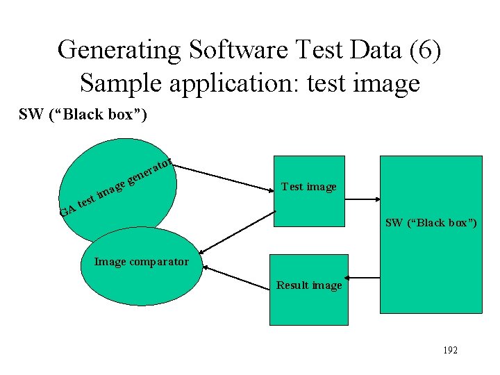
Generating Software Test Data (6) Sample application: test image SW (“Black box”) tor a r ne e t GA e m st i g age Test image SW (“Black box”) Image comparator Result image 192

Generating Software Test Data (7) Co-evolutionary SW testing and development: Ø Co-evolutionary SW testing and development: optimizing and testing surface measurement software Ø One GA generates test surfaces to test the error bounds of the measurement software Ø Another GA is simultaneously developing the SW parameters in order to achieve better accuracy 193

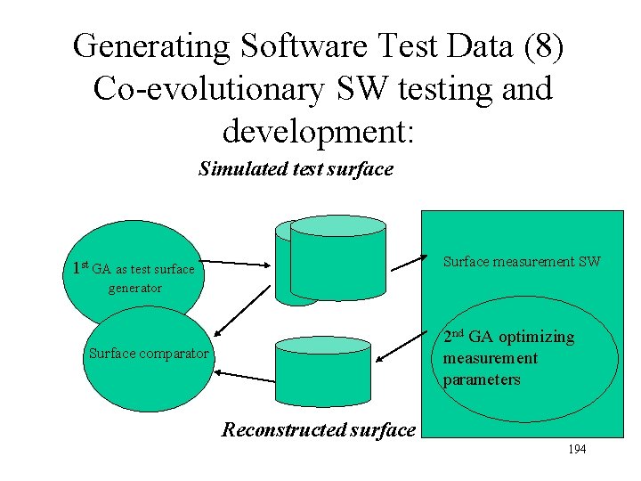
Generating Software Test Data (8) Co-evolutionary SW testing and development: Simulated test surface Surface measurement SW 1 st GA as test surface generator 2 nd GA optimizing measurement parameters Surface comparator Reconstructed surface 194

Multi-objective optimization (1) • For many problems there is a need for simultaneous optimization of multiple objectives. It is clear that if, for example, two objectives are to be optimized, it might be possible to find a solution which is best with respect to the first solution and, and another solution, which is best with respect to the second objective. • Examples: Ø To maximize profit of the company and to increase company prestige. Ø To maximize a function f(x) in a domain D and simultaneously to minimize another function ff(x). 195

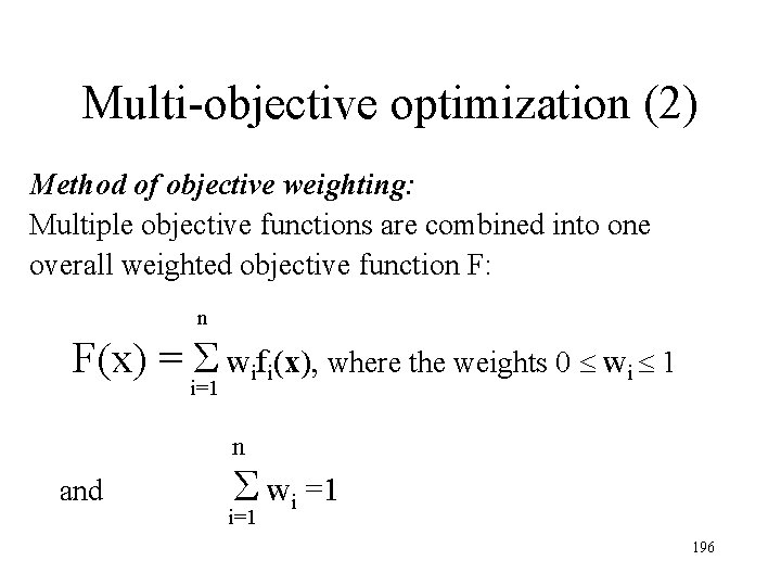
Multi-objective optimization (2) Method of objective weighting: Multiple objective functions are combined into one overall weighted objective function F: n F(x) = Σ wifi(x), where the weights 0 wi 1 i=1 n and Σ wi =1 i=1 196

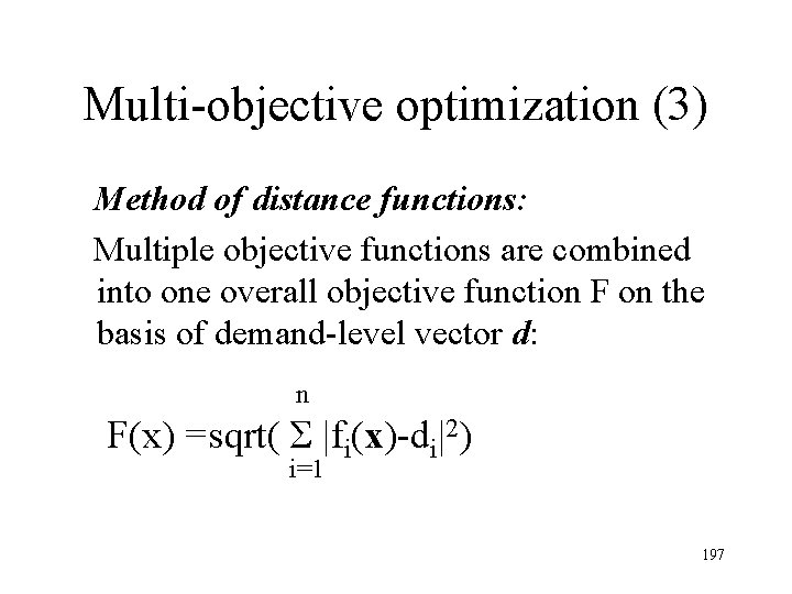
Multi-objective optimization (3) Method of distance functions: Multiple objective functions are combined into one overall objective function F on the basis of demand-level vector d: n F(x) =sqrt( Σ |fi(x)-di|2) i=1 197

Hybrid approach (1) Two major types of hybrid GA methods: • Internal GA hybrid methods where GA is employed as a driver of a broader iterative optimization process • External GA hybrid methods where GA is employed to get an initial point for another, local optimization method 198

Hybrid approach (2) Internal GA: Usually applied where the calculation of objective function is very expensive and surrogate (approximate) estimations computations are used instead. In this case, it is necessary to iterate GA search verifying the result at the end of each iteration by accurate estimate of the objective function and using the current “optimal” solution as an initial point for the next iteration. 199

Hybrid approach (3) External GA: Usually applied in order to come closer to the optimum. In this case, the GA suboptimal solution serves as an initial point for a local but accurate optimization method (e. g. gradient method) 200