GENETIC ALGORITHMS AND LINEAR DISCRIMINANT ANALYSIS BASED DIMENSIONALITY

GENETIC ALGORITHMS AND LINEAR DISCRIMINANT ANALYSIS BASED DIMENSIONALITY REDUCTION FOR REMOTELY SENSED IMAGE ANALYSIS Minshan Cui, Saurabh Prasad, Majid Mahroogy, Lori Mann Bruce, James Aanstoos

Traditional Approaches (Stepwise Selection, Greedy Search, …) § Stepwise LDA (S-LDA), (DAFE) • A preliminary forward selection and backward rejection is employed to discard less relevant features. • A Linear Discriminant Analysis (LDA) projection is applied on this reduced subset of features to further reduce the dimensionality of the feature space. § Drawbacks • In forward selection, one is unable to reevaluate the features that become irrelevant after adding some other features. • In backward rejection, one is unable to reevaluate the features after they have been discarded.

Genetic Algorithm § Genetic algorithms are a class of optimization techniques that search for the global minimum of a fitness function. § This typically involves four steps – evaluation, reproduction, recombination, and mutation.

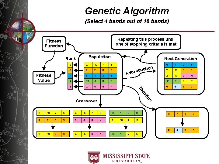
Genetic Algorithm (Select 4 bands out of 10 bands) Repeating this process until one of stopping criteria is met Fitness Function Population Rank Fitness Value Next Generation 2 10 7 5 5 1 2 8 3 9 7 8 3 2 10 8 3 1 5 1 2 8 2 10 9 4 4 10 4 3 6 10 4 7 5 5 2 5 9 4 9 5 8 3 R ction u d o epr io at ut M 2 n Crossover 2 10 7 5 10 4 3 6 9 7 8 3 2 5 9 4 2 10 7 5 2 10 8 3 2 10 9 4 10 4 7 5 9 7 8 3 9 5 8 3

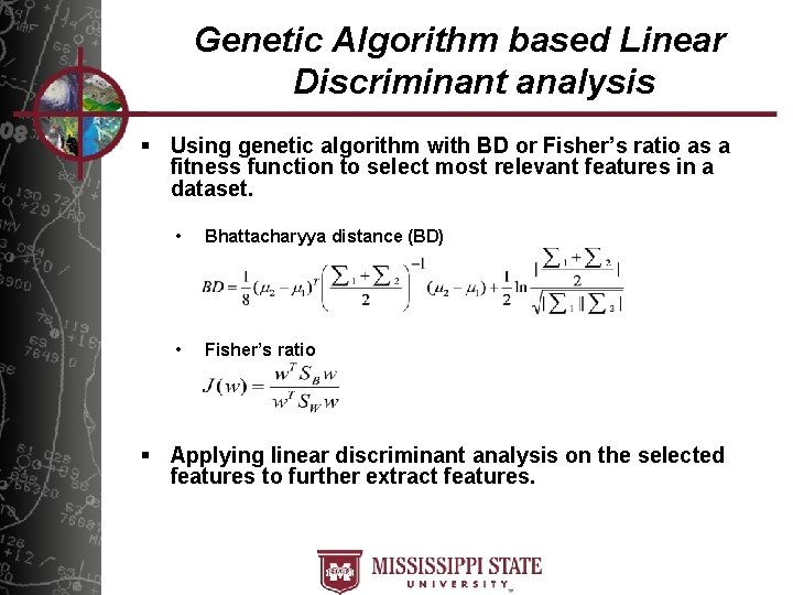
Genetic Algorithm based Linear Discriminant analysis § Using genetic algorithm with BD or Fisher’s ratio as a fitness function to select most relevant features in a dataset. • Bhattacharyya distance (BD) • Fisher’s ratio § Applying linear discriminant analysis on the selected features to further extract features.

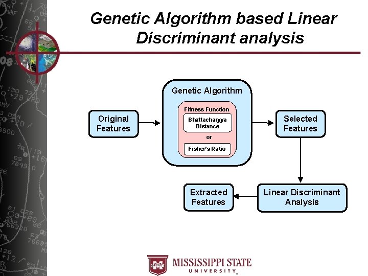
Genetic Algorithm based Linear Discriminant analysis Genetic Algorithm Fitness Function Original Features Bhattacharyya Distance Selected Features or Fisher’s Ratio Extracted Features Linear Discriminant Analysis

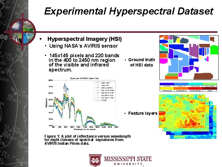
Experimental Hyperspectral Dataset § Hyperspectral Imagery (HSI) • Using NASA’s AVIRIS sensor • 145 x 145 pixels and 220 bands • Ground truth in the 400 to 2450 nm region of HSI data of the visible and infrared spectrum. • Feature layers Figure 1: A plot of reflectance versus wavelength for eight classes of spectral signatures from AVIRIS Indian Pines data.

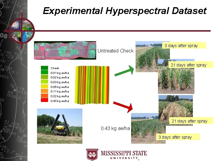
Experimental Hyperspectral Dataset 3 days after spray Untreated Check 21 days after spray Check 0. 01 kg ae/ha 0. 02 kg ae/ha 0. 03 kg ae/ha 0. 05 kg ae/ha 0. 11 kg ae/ha 0. 22 kg ae/ha 0. 43 kg ae/ha 21 days after spray 0. 43 kg ae/ha 3 days after spray

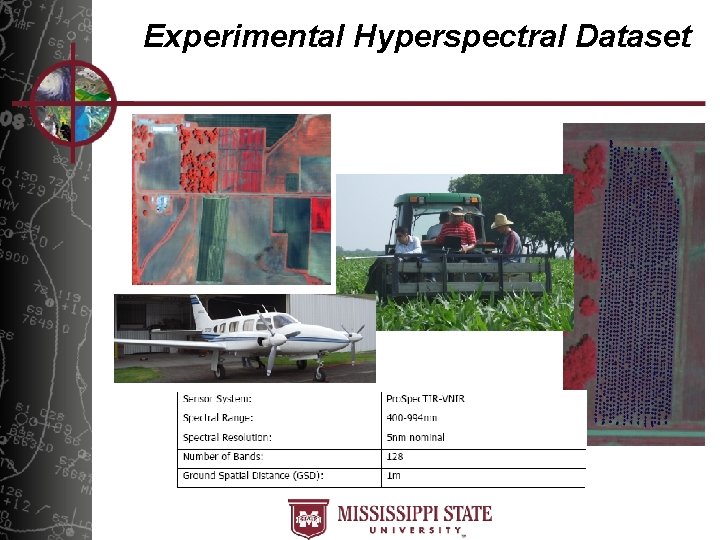
Experimental Hyperspectral Dataset

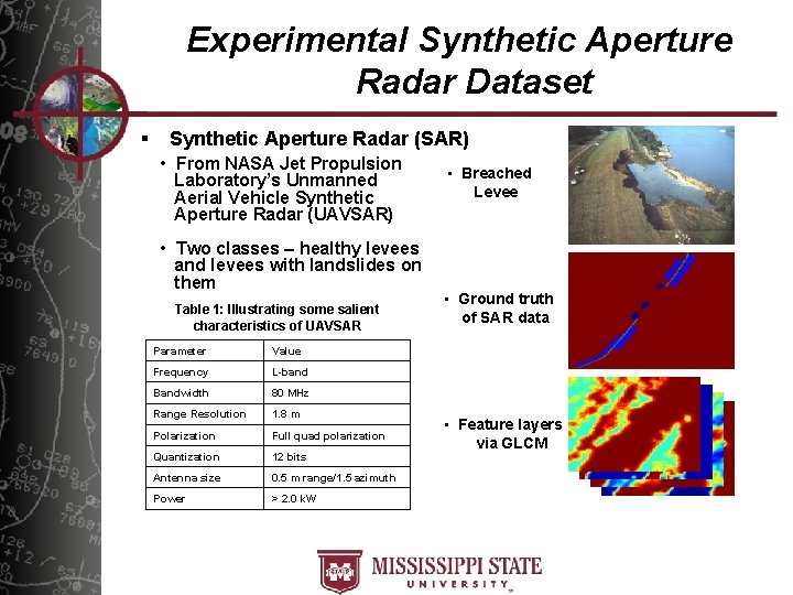
Experimental Synthetic Aperture Radar Dataset § Synthetic Aperture Radar (SAR) • From NASA Jet Propulsion Laboratory’s Unmanned Aerial Vehicle Synthetic Aperture Radar (UAVSAR) • Two classes – healthy levees and levees with landslides on them Table 1: Illustrating some salient characteristics of UAVSAR Parameter Value Frequency L-band Bandwidth 80 MHz Range Resolution 1. 8 m Polarization Full quad polarization Quantization 12 bits Antenna size 0. 5 m range/1. 5 azimuth Power > 2. 0 k. W • Breached Levee • Ground truth of SAR data • Feature layers via GLCM

Experiments § HSI and SAR analysis using: • LDA • Stepwise LDA (S-LDA) • GA-LDA-Fisher (Using Fisher’s ratio as a fitness function in GA. ) • GA-LDA-BD (Using Bhattacharyya distance as a fitness function in GA. ) § Performance measures: • Overall recognition accuracies

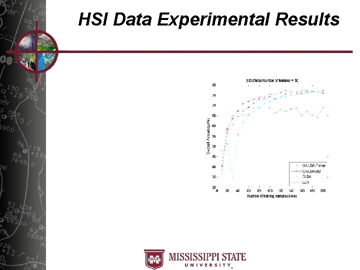
HSI Data Experimental Results

SAR Data Experimental Results

Conclusions § GA search is very effective at selecting the most pertinent features. § Given a moderate feature space dimensionality and sufficient training samples, LDA is a good projection based dimensionality reduction strategy. § As the number of features increases and the trainingsample-size decreases, methods such as GA-LDA can assist by providing a robust intermediate step of pruning away redundant and less useful features.

References [1] Ho-Duck Kim, Chang-Hyun Park, Hyun-Chang Yang, Kwee-Bo Sim, “Genetic Algorithm Based Feature Selection Method Development for Pattern Recognition, ” in SICE-ICASE, 2006. [2] Chulhee Lee and Daesik Hong, “Feature Extraction Using the Bhattacharyya Distance, ” in IEEE International on Systems, Man, and Cybernetics, 1997 [3] Tran Huy Dat, Cuntai Guan, “Feature selection based on fisher ratio and mutual information analysis for robust brain computer interface, ” in IEEE International Conference on Acoustics, Speech and Signal Processing, 2007. [4] R. O. Duda, P. E. Stark, D. G. Stork, Pattern Classification, Wiley Inter-science, October 2000. [5] S. Prasad and L. M. Bruce, “Limitations of Principal Components Analysis for Hyperspectral Target Recognition, ” in IEEE Geoscience and Remote Sensing Letters, vol. 5, pp. 625 -629, 2008. [6] S. Kumar, J. Ghosh, M. M. Crawford, “Best-bases feature extraction algorithms for classification of hyperspectral data, ” in IEEE Transactions on Geoscience and Remote Sensing, Vol. 39, No. 7, pp 13681379, July 2001. [7] Nakariyakul, S. , Casasent, D. P. , “Improved forward floating selection algorithm for feature subset selection, ” in Proceedings of the 2008 International Conference on Wavelet Analysis and Pattern Recognition, Hong. Kong, 30 -31 Aug. 2008. [8] K. S. Tang, K. F. Man, S. Kwong, Q. He, “Genetic algorithms and their applications, ” in IEEE Signal Processing Magazine, Vol. 13, Nov 1996. [9] NASA Jet Propulsion Laboratory Airborne Visible/Infrared Imaging Spectrometer (AVIRIS) web page http: //aviris. jpl. nasa. gov/ [10] Kevin Wheeler, Scott Hensley, Yunling Lou, Tim Miller, Jim Hoffman, "An L-band SAR for repeat pass deformation measurements on a UAV platform", 2004 IEEE Radar Conference, Philadelphia, PA, April 2004. (classifying health levee from landslide in a UAVSAR image).

Thank You Questions - Comments - Suggestions Minshan Cui minshan@gri. msstate. edu

How many elite, crossover and mutate kids will be produced in next generation? § Elite count Specifies the number of individuals that are guaranteed to survive to the next generation. § Crossover fraction Specifies the fraction of the next generation, other than elite children, that are produced by crossover. § Ex) Assume population size =10, elite count = 2 and crossover fraction = 0. 8 • • • n. Elite. Kids = 2 n. Crossover. Kids = round(Crossover. Fraction × (10 - n. Elite. Kids)) = round( 0. 8 × (10 – 2)) = 6 n. Mutate. Kids = 10 - n. Elite. Kids - n. Crossover. Kids = 10 - 2 - 6 = 2

How many parents GA need to produce crossover kids and mutate kids? § Since 2 parents produce 1 crossover kid and 1 parent produce 1 mutate kid, GA will need: n. Parents = 2 × n. Crossover. Kids + n. Mutate. Kids = 2 × 6 + 2 = 14. § GA will need 12 parents to produce 6 crossover kids and 2 parents to produce 2 mutate kids.

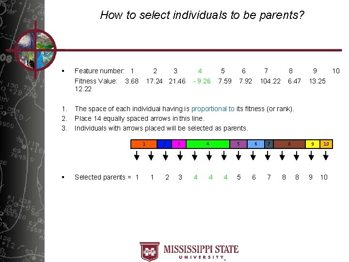
How to select individuals to be parents? § Feature number: 1 Fitness Value: 3. 68 12. 22 1. 2. 3. The space of each individual having is proportional to its fitness (or rank). Place 14 equally spaced arrows in this line. Individuals with arrows placed will be selected as parents. 2 3 17. 24 21. 46 1 § Selected parents = 1 2 4 - 9. 26 3 3 5 7. 59 4 4 6 7. 92 7 104. 22 5 6 7 8 6. 47 8 8 8 9 10 13. 25 9 10

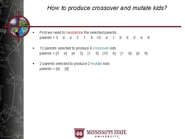
How to produce crossover and mutate kids? § § § First we need to randomize the selected parents = 3 4 4 2 1 5 10 4 1 8 12 parents selected to produce 6 crossover kids. parents = [3 4] [4 2] [1 5] [10 4] [1 2 parents selected to produce 2 mutate kids. parents = [6] [8] 6 8] 9 6 [6 8 9]

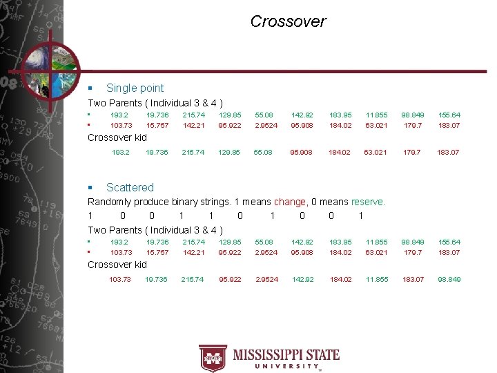
Crossover § Single point Two Parents ( Individual 3 & 4 ) • • 193. 2 103. 73 19. 736 15. 757 215. 74 142. 21 129. 85 95. 922 55. 08 2. 9524 142. 92 95. 908 183. 95 184. 02 11. 855 63. 021 98. 849 179. 7 155. 64 183. 07 215. 74 129. 85 55. 08 95. 908 184. 02 63. 021 179. 7 183. 07 Crossover kid 193. 2 § 19. 736 Scattered Randomly produce binary strings. 1 means change, 0 means reserve. 1 0 0 1 Two Parents ( Individual 3 & 4 ) • • 193. 2 103. 73 19. 736 15. 757 215. 74 142. 21 129. 85 95. 922 55. 08 2. 9524 142. 92 95. 908 183. 95 184. 02 11. 855 63. 021 98. 849 179. 7 155. 64 183. 07 215. 74 95. 922 2. 9524 142. 92 184. 02 11. 855 183. 07 98. 849 Crossover kid 103. 73 19. 736

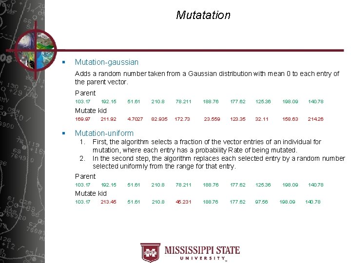
Mutatation § Mutation-gaussian Adds a random number taken from a Gaussian distribution with mean 0 to each entry of the parent vector. Parent 103. 17 192. 15 51. 61 210. 8 78. 211 188. 76 177. 62 125. 36 198. 09 140. 78 4. 7027 82. 935 172. 73 23. 559 123. 35 32. 11 158. 63 214. 26 Mutate kid 169. 97 § 211. 92 Mutation-uniform 1. First, the algorithm selects a fraction of the vector entries of an individual for mutation, where each entry has a probability Rate of being mutated. 2. In the second step, the algorithm replaces each selected entry by a random number selected uniformly from the range for that entry. Parent 103. 17 192. 15 51. 61 210. 8 78. 211 188. 76 177. 62 125. 36 51. 61 210. 8 45. 231 188. 76 177. 62 97. 56 198. 09 140. 78 Mutate kid 103. 17 213. 45 198. 09 140. 78

Next generation § next. Generation = [ elite. Kids, crossover. Kids, mutate. Kids ]

Stopping criteria 1. Generations — Specifies the maximum number of iterations for the genetic algorithm to perform. The default is 100. 2. Time limit — Specifies the maximum time in seconds the genetic algorithm runs before stopping. 3. Fitness limit — The algorithm stops if the best fitness value is less than or equal to the value of Fitness limit. 4. Stall generations — The algorithm stops if the weighted average change in the fitness function value over Stall generations is less than Function tolerance. 5. Stall time limit — The algorithm stops if there is no improvement in the best fitness value for an interval of time in seconds specified by Stall time. 6. Function tolerance — The algorithm runs until the cumulative change in the fitness function value over Stall generations is less than or equal to Function Tolerance.