Generative Models for Image Understanding Nebojsa Jojic and

Generative Models for Image Understanding Nebojsa Jojic and Thomas Huang Beckman Institute and ECE Dept. University of Illinois

Problem: Summarization of High Dimensional Data • Pattern Analysis: – For several classes c=1, . . , C of the data, define probability distribution functions p(x| c) • Compression: – Define a probabilistic model p(x) and devise an optimal coding approach • Video Summary: – Drop most of the frames in a video sequence and keep interesting information that summarizes it.

Generative density modeling • Find a probability model that – reflects desired structure – randomly generates plausible images, – represents the data by parameters • ML estimation • p(image|class) used for recognition, detection, . . .

Problems we attacked • Transformation as a discrete variable in generative models of intensity images • Tracking articulated objects in dense stereo maps • Unsupervised learning for video summary • Idea - the structure of the generative model reveals the interesting objects we want to extract.

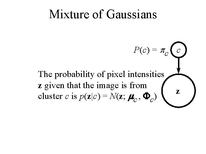
Mixture of Gaussians P(c) = pc c The probability of pixel intensities z given that the image is from cluster c is p(z|c) = N(z; mc , Fc) z

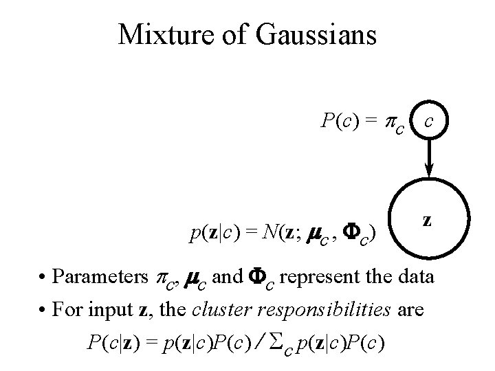
Mixture of Gaussians P(c) = pc c p(z|c) = N(z; mc , Fc) z • Parameters pc, mc and Fc represent the data • For input z, the cluster responsibilities are P(c|z) = p(z|c)P(c) / Sc p(z|c)P(c)

Example: Simulation p 1= 0. 6, m 1= F 1= p 2= 0. 4, m 2= F 2= P(c) = pc c=1 z= p(z|c) = N(z; mc , Fc)

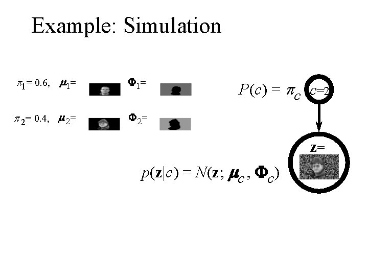
Example: Simulation p 1= 0. 6, m 1= F 1= p 2= 0. 4, m 2= F 2= P(c) = pc c=2 z= p(z|c) = N(z; mc , Fc)

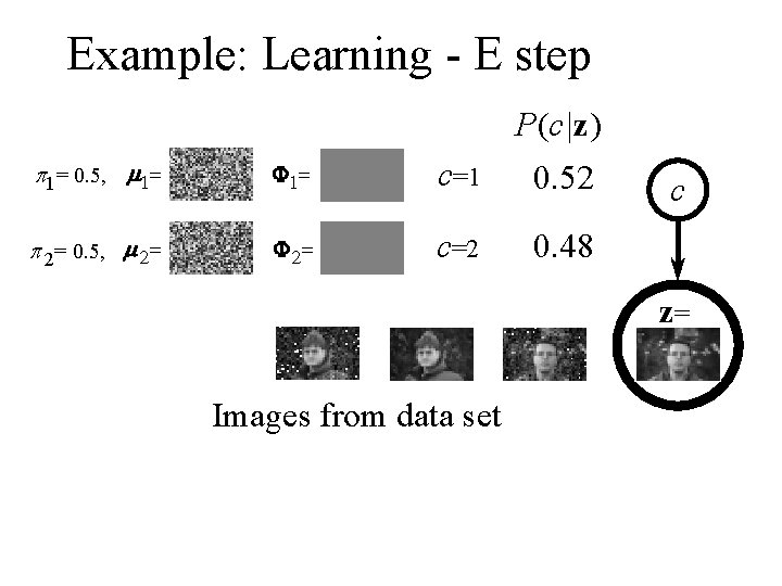
Example: Learning - E step P(c|z) p 1= 0. 5, m 1= F 1= c=1 0. 52 p 2= 0. 5, m 2= F 2= c=2 0. 48 c z= Images from data set

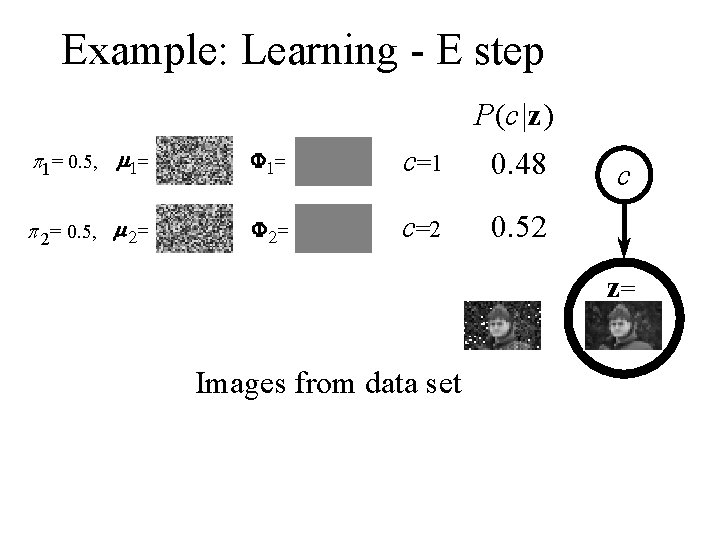
Example: Learning - E step P(c|z) p 1= 0. 5, m 1= F 1= c=1 0. 48 p 2= 0. 5, m 2= F 2= c=2 0. 52 c z= Images from data set

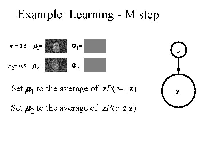
Example: Learning - M step p 1= 0. 5, m 1= F 1= p 2= 0. 5, m 2= F 2= Set m 1 to the average of z. P(c=1|z) Set m 2 to the average of z. P(c=2|z) c z

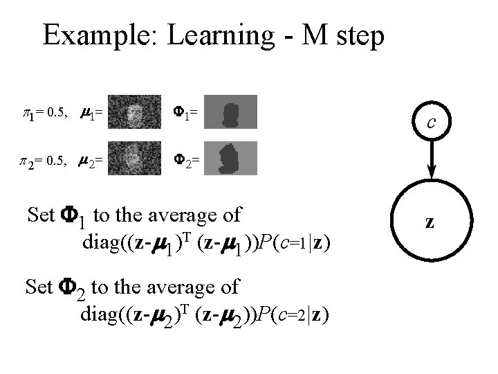
Example: Learning - M step p 1= 0. 5, m 1= F 1= p 2= 0. 5, m 2= F 2= Set F 1 to the average of diag((z-m 1)T (z-m 1))P(c=1|z) Set F 2 to the average of diag((z-m 2)T (z-m 2))P(c=2|z) c z

Transformation as a Discrete Latent Variable with Brendan J. Frey Computer Science, University of Waterloo, Canada Beckman Institute & ECE, Univ of Illinois at Urbana

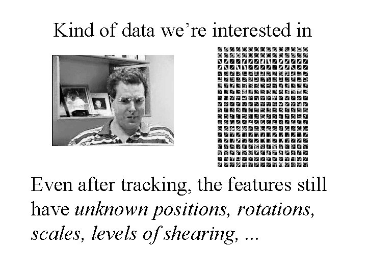
Kind of data we’re interested in Even after tracking, the features still have unknown positions, rotations, scales, levels of shearing, . . .

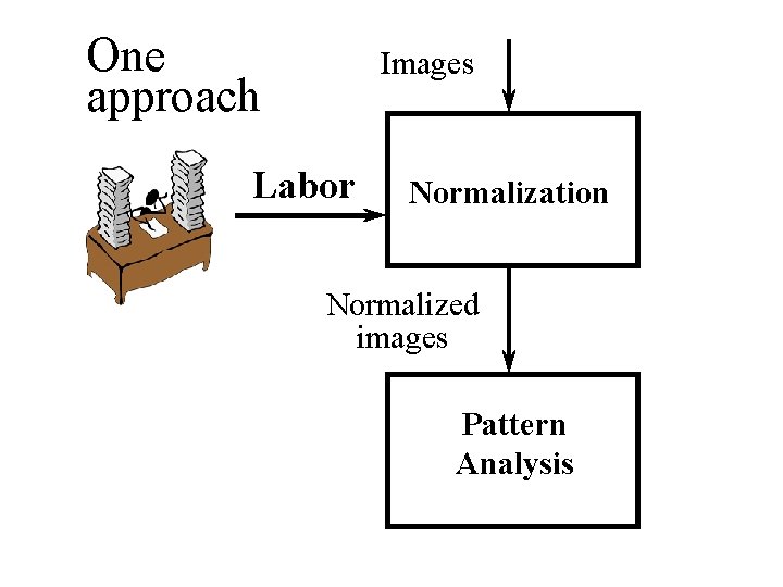
One approach Images Labor Normalization Normalized images Pattern Analysis

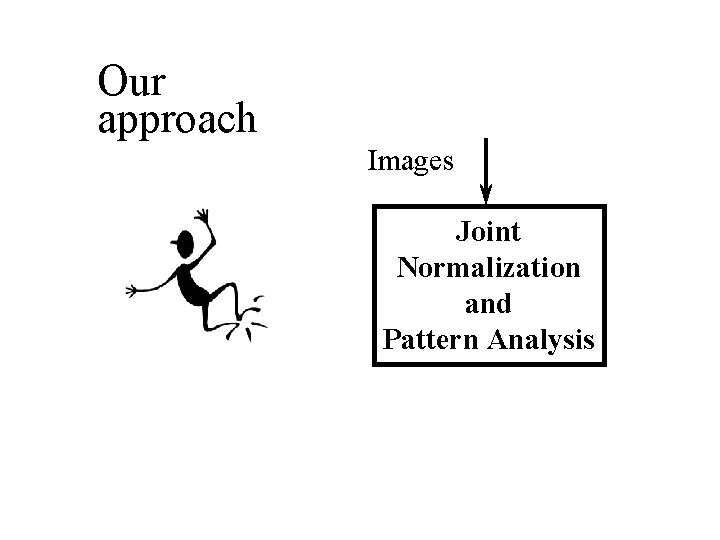
Our approach Images Joint Normalization and Pattern Analysis

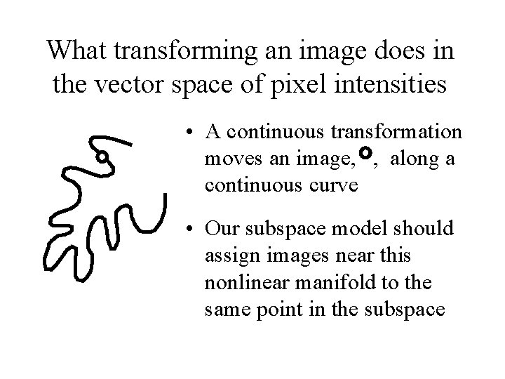
What transforming an image does in the vector space of pixel intensities • A continuous transformation moves an image, , along a continuous curve • Our subspace model should assign images near this nonlinear manifold to the same point in the subspace

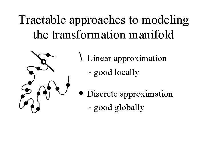
Tractable approaches to modeling the transformation manifold Linear approximation - good locally • Discrete approximation - good globally

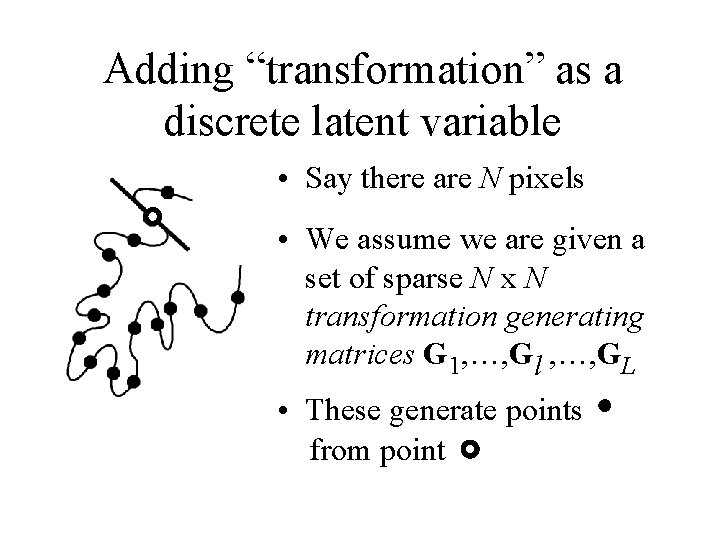
Adding “transformation” as a discrete latent variable • Say there are N pixels • We assume we are given a set of sparse N x N transformation generating matrices G 1, …, Gl , …, GL • These generate points from point

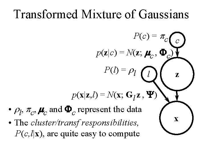
Transformed Mixture of Gaussians P(c) = pc c p(z|c) = N(z; mc , Fc) P(l) = rl l z p(x|z, l) = N(x; Gl z , Y) • rl, pc, mc and Fc represent the data • The cluster/transf responsibilities, P(c, l|x), are quite easy to compute x

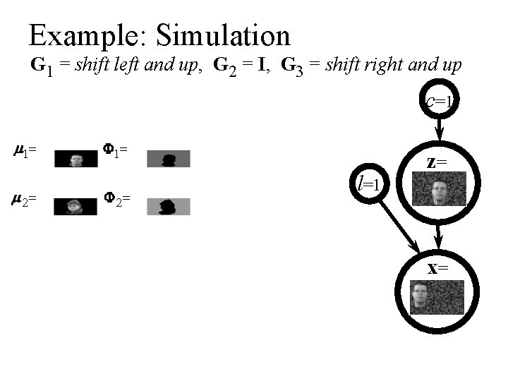
Example: Simulation G 1 = shift left and up, G 2 = I, G 3 = shift right and up c=1 m 1= m 2= F 1= F 2= l=1 z= x=

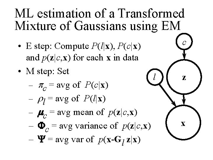
ML estimation of a Transformed Mixture of Gaussians using EM • E step: Compute P(l|x), P(c|x) and p(z|c, x) for each x in data • M step: Set l – pc = avg of P(c|x) – rl = avg of P(l|x) – mc = avg mean of p(z|c, x) – Fc = avg variance of p(z|c, x) – Y = avg var of p(x-Gl z|x) c z x

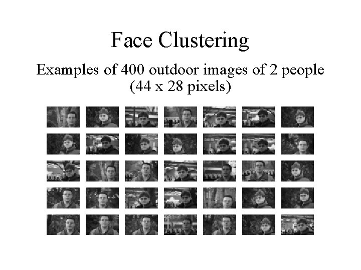
Face Clustering Examples of 400 outdoor images of 2 people (44 x 28 pixels)

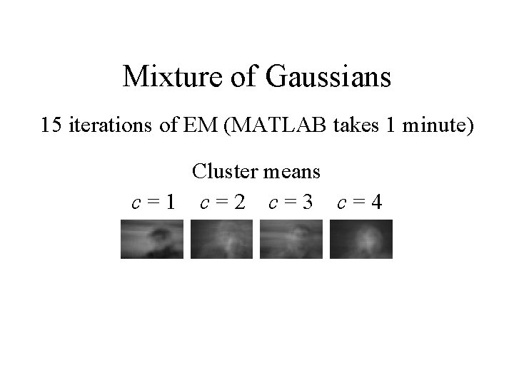
Mixture of Gaussians 15 iterations of EM (MATLAB takes 1 minute) Cluster means c=1 c=2 c=3 c=4

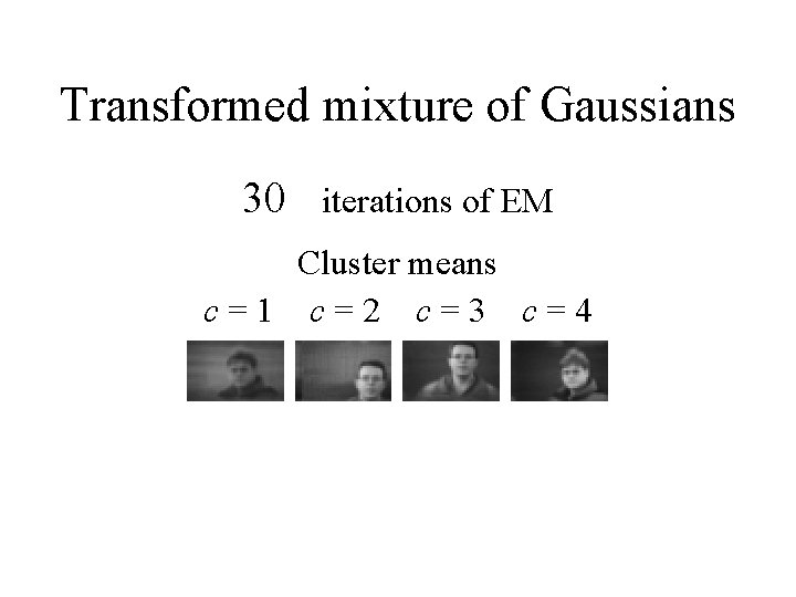
Transformed mixture of Gaussians 30 iterations of EM Cluster means c=1 c=2 c=3 c=4

Video Analysis Using Generative Models with Brendan Frey, Nemanja Petrovic and Thomas Huang

Idea • Use generative models of video sequences to do unsupervised learning • Use the resulting model for video summarization, filtering, stabilization, recognition of objects, retrieval, etc.

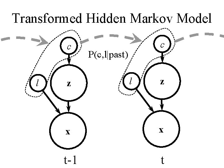
Transformed Hidden Markov Model c l z c P(c, l|past) l z x x t-1 t

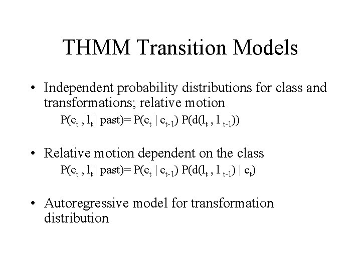
THMM Transition Models • Independent probability distributions for class and transformations; relative motion P(ct , lt | past)= P(ct | ct-1) P(d(lt , l t-1)) • Relative motion dependent on the class P(ct , lt | past)= P(ct | ct-1) P(d(lt , l t-1) | ct) • Autoregressive model for transformation distribution

Inference in THMM • Tasks: – Find the most likely state at time t given the whole observed sequence {xt} and the model parameters (class means and variances, transition probabilities, etc. ) – Find the distribution over states for each time t – Find the most likely state sequence – Learn the parameters that maximize he likelihood of the observed data

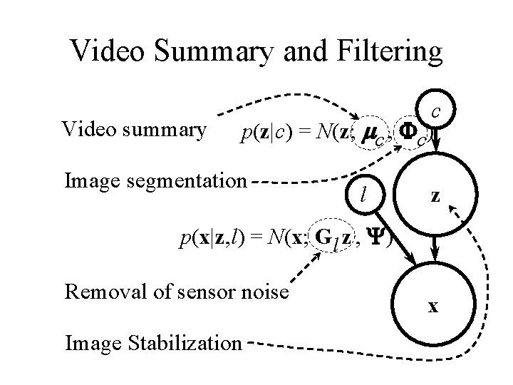
Video Summary and Filtering Video summary c p(z|c) = N(z; mc , Fc) Image segmentation l z p(x|z, l) = N(x; Gl z , Y) Removal of sensor noise Image Stabilization x

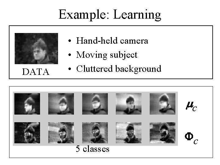
Example: Learning DATA • Hand-held camera • Moving subject • Cluttered background mc 1 class 121 translations (11 vertical and 11 horizontal shifts) Fc 5 classes mc Fc

Examples • Normalized sequence • Simulated sequence • De-noising • Seeing through distractions

Future work • Fast approximate learning and inference • Multiple layers • Learning transformations from images Nebojsa Jojic: www. ifp. uiuc. edu/~jojic

Subspace models of images Example: Image, R 1200 = f (y, R 2) Shut eyes Frown

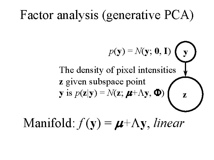
Factor analysis (generative PCA) p(y) = N(y; 0, I) y The density of pixel intensities z given subspace point y is p(z|y) = N(z; m+Ly, F) z Manifold: f (y) = m+Ly, linear

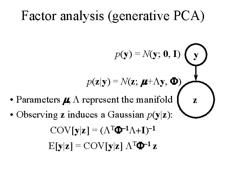
Factor analysis (generative PCA) p(y) = N(y; 0, I) y p(z|y) = N(z; m+Ly, F) • Parameters m, L represent the manifold • Observing z induces a Gaussian p(y|z): COV[y|z] = (LTF-1 L+I)-1 E[y|z] = COV[y|z] LTF-1 z z

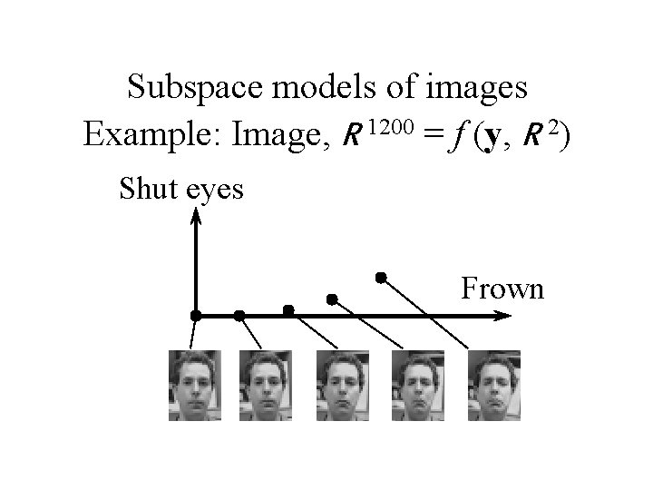
Shut eyes L= Frown Example: Simulation m= SE p(y) = N(y; 0, I) y Frn p(z|y) = N(z; m+Ly, F) z

Shut eyes L= Frown Example: Simulation m= SE p(y) = N(y; 0, I) y Frn p(z|y) = N(z; m+Ly, F) z

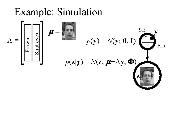
Shut eyes L= Frown Example: Simulation m= SE p(y) = N(y; 0, I) y Frn p(z|y) = N(z; m+Ly, F) z

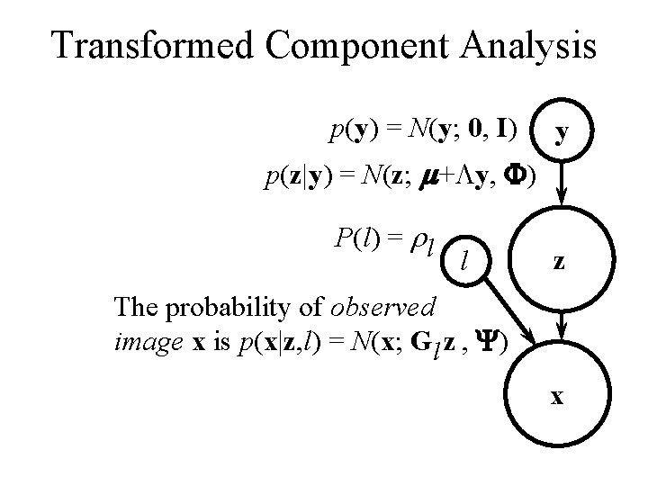
Transformed Component Analysis p(y) = N(y; 0, I) y p(z|y) = N(z; m+Ly, F) P(l) = rl l z The probability of observed image x is p(x|z, l) = N(x; Gl z , Y) x

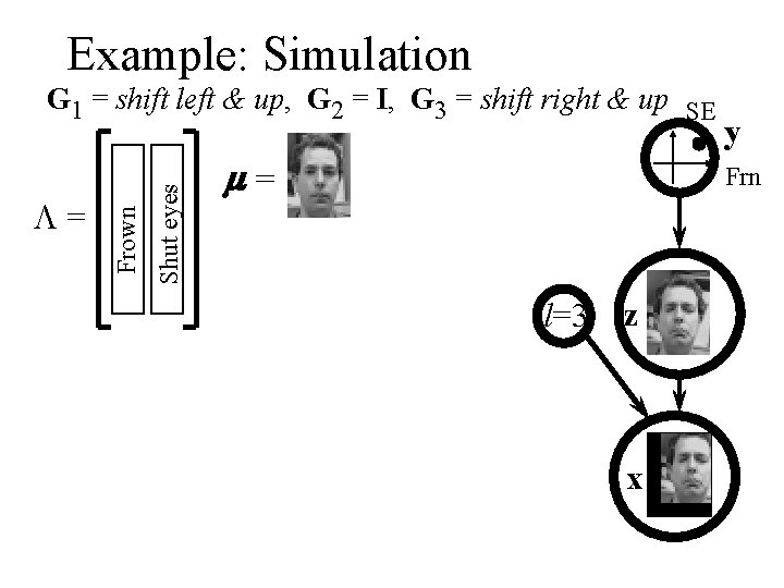
Example: Simulation Shut eyes L= Frown G 1 = shift left & up, G 2 = I, G 3 = shift right & up SE m= y Frn l=3 z x

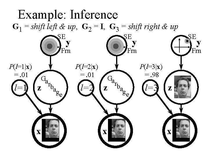
Example: Inference G 1 = shift left & up, G 2 = I, G 3 = shift right & up SE SE y Frn P(l=1|x) =. 01 l=1 Ga z rbag e x y Frn P(l=2|x) =. 01 l=2 Ga rb z ag e x SE y Frn P(l=3|x) =. 98 l=3 z x

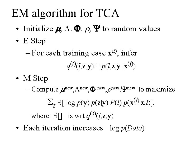
EM algorithm for TCA • Initialize m, L, F, r, Y to random values • E Step – For each training case x(t), infer q(t)(l, z, y) = p(l, z, y |x(t)) • M Step – Compute mnew, Lnew, F new, rnew, Ynew to maximize St E[ log p(y) p(z|y) P(l) p(x(t)|z, l)], where E[] is wrt q(t)(l, z, y) • Each iteration increases log p(Data)

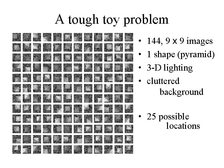
A tough toy problem • • 144, 9 x 9 images 1 shape (pyramid) 3 -D lighting cluttered background • 25 possible locations

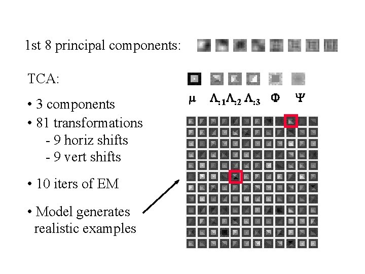
1 st 8 principal components: TCA: • 3 components • 81 transformations - 9 horiz shifts - 9 vert shifts • 10 iters of EM • Model generates realistic examples m L: 1 L: 2 L: 3 F Y

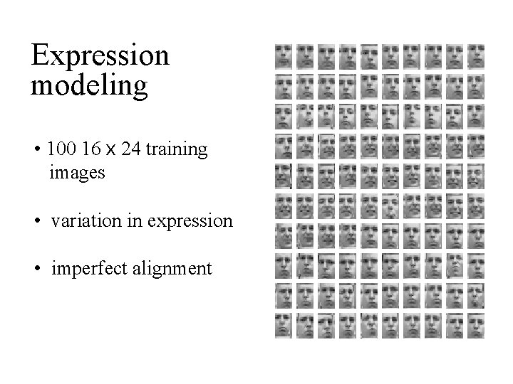
Expression modeling • 100 16 x 24 training images • variation in expression • imperfect alignment

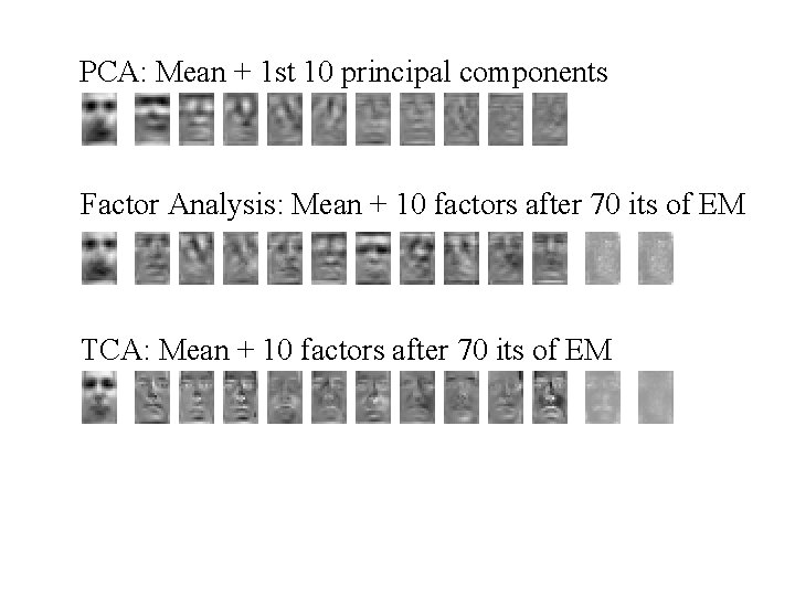
PCA: Mean + 1 st 10 principal components Factor Analysis: Mean + 10 factors after 70 its of EM TCA: Mean + 10 factors after 70 its of EM

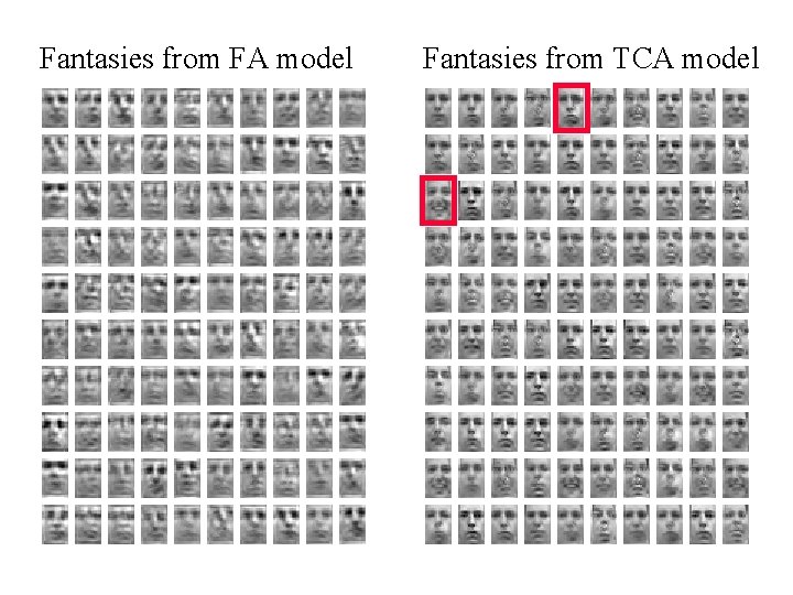
Fantasies from FA model Fantasies from TCA model

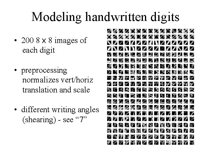
Modeling handwritten digits • 200 8 x 8 images of each digit • preprocessing normalizes vert/horiz translation and scale • different writing angles (shearing) - see “ 7”

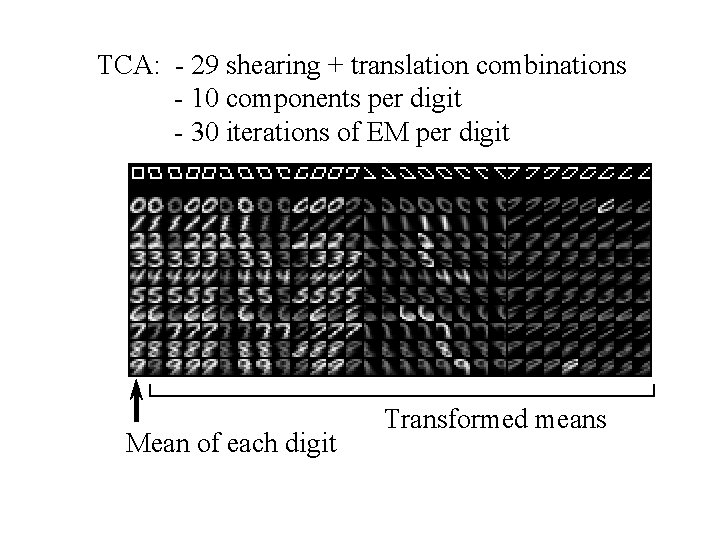
TCA: - 29 shearing + translation combinations - 10 components per digit - 30 iterations of EM per digit Mean of each digit Transformed means

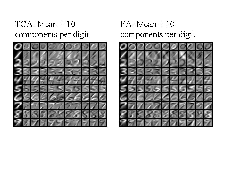
TCA: Mean + 10 components per digit FA: Mean + 10 components per digit

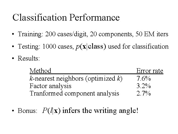
Classification Performance • Training: 200 cases/digit, 20 components, 50 EM iters • Testing: 1000 cases, p(x|class) used for classification • Results: Method k-nearest neighbors (optimized k) Factor analysis Tranformed component analysis Error rate 7. 6% 3. 2% 2. 7% • Bonus: P(l|x) infers the writing angle!

Wrap-up • Papers, MATLAB scripts: www. ifp. uiuc. edu/~jojic www. cs. uwaterloo. ca/~frey • Other domains: audio, bioinfomatics, … • Other latent image models, p(z) – mixtures of factor analyzers (NIPS 99) – layers, multiple objects, occlusions – time series (in preparation)

Wrap-up • Discrete+Linear Combination: Set some components equal to derivatives of m wrt transformations • Multiresolution approach • Fast variational methods, belief propagation, . . .

Other generative models • Modeling human appearance in stereo images: articulated, self-occluding Gaussians