Generative adversarial networks GANs Kh wong Generative adversarial

Generative adversarial networks (GANs) Kh wong Generative adversarial networks (GAN) (v 0. 1. a) 1

Overview 1) 2) 3) 4) Introduction Theory Example Case study: GAN for edge detection Generative adversarial networks (GAN) (v 0. 1. a) 2

1) Introduction • Non-supervised learning • Require 2 Convolution neural networks: Generator (G) and discriminator (D) • Training of GANs Use Generator (G) to generate noise Use the noise to generate data A discriminator (D) to determine it is true or false Update the neural networks until the discriminator cannot tell whether the generator is producing true or false data – After trained G, G can generate many more training samples for training of other neural network algorithms – – Generative adversarial networks (GAN) (v 0. 1. a) 3

2) Theory of Generative adversarial networks (GANs) Idea and math Generative adversarial networks (GAN) (v 0. 1. a) 4

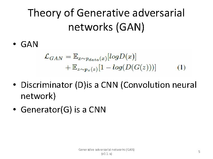
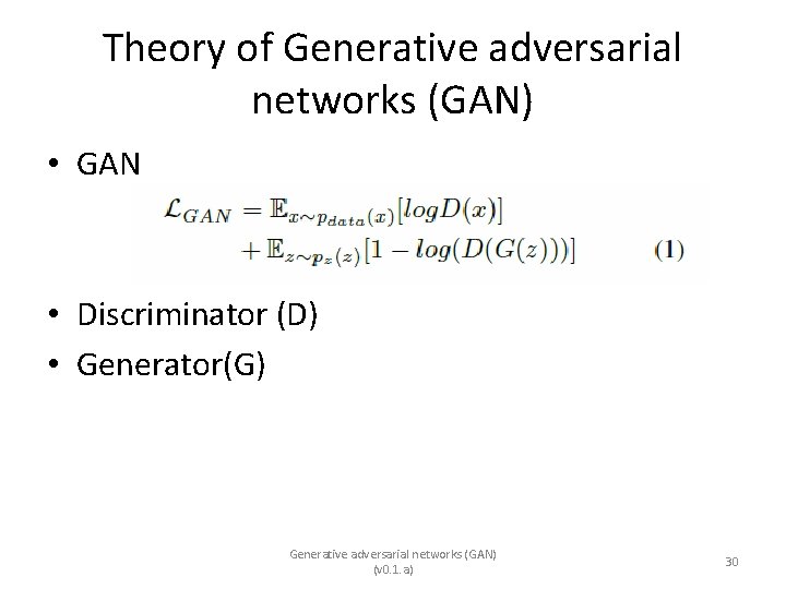
Theory of Generative adversarial networks (GAN) • GAN • Discriminator (D)is a CNN (Convolution neural network) • Generator(G) is a CNN Generative adversarial networks (GAN) (v 0. 1. a) 5

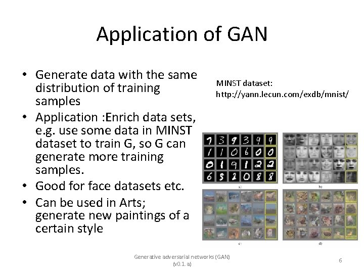
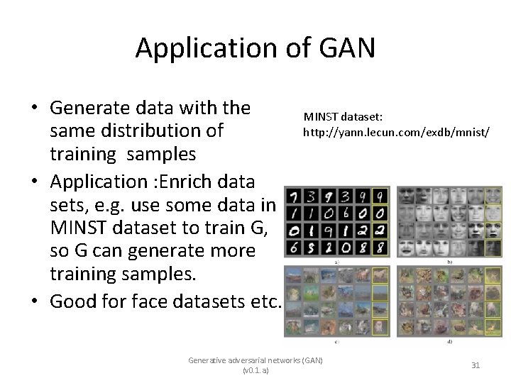
Application of GAN • Generate data with the same distribution of training samples • Application : Enrich data sets, e. g. use some data in MINST dataset to train G, so G can generate more training samples. • Good for face datasets etc. • Can be used in Arts; generate new paintings of a certain style MINST dataset: http: //yann. lecun. com/exdb/mnist/ Generative adversarial networks (GAN) (v 0. 1. a) 6

The idea, from : Goodfellow, Ian, et al. "Generative adversarial nets. " Advances in neural information processing systems. 2014. https: //arxiv. org/abs/1406. 2661 • The proposed adversarial nets framework, the generative model is pitted against an adversary: • a discriminative model (D) that learns to determine whether a sample is from the model distribution or the data distribution. The generative model (G) can be thought of as analogous to a team of counterfeiters, trying to produce fake currency and use it without detection, while the discriminative model is analogous to the police, trying to detect the counterfeit currency. Competition in this game drives both teams to improve their methods until the counterfeits are indistinguishable from the genuine articles. Generative adversarial networks (GAN) (v 0. 1. a) 7

GAN algorithm • Part 1: The Discriminator is trained while the Generator is idle. In this phase, the (Generator) network is only forward propagated and no back-propagation is done. The Discriminator is trained (with back-progataion) on real data for n epochs, and see if it can correctly predict them as real. Also, in this phase, the Discriminator is also trained on the fake generated data from the Generator and see if it can correctly predict them as fake. • Part 2: The Generator (with backpropagation) is trained while the Discriminator is idle. After the Discriminator is trained by the generated fake data of the Generator, we can get its predictions and use the results for training the Generator and get better from the previous state to try and fool the Discriminator. • https: //www. geeksforgeeks. org/generative-adversarial-networkgan/ Generative adversarial networks (GAN) (v 0. 1. a) 8

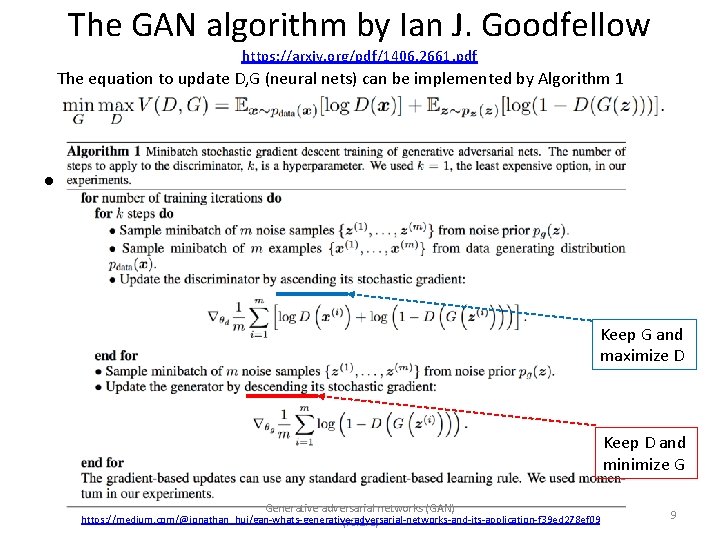
The GAN algorithm by Ian J. Goodfellow https: //arxiv. org/pdf/1406. 2661. pdf The equation to update D, G (neural nets) can be implemented by Algorithm 1 • Keep G and maximize D Keep D and minimize G Generative adversarial networks (GAN) https: //medium. com/@jonathan_hui/gan-whats-generative-adversarial-networks-and-its-application-f 39 ed 278 ef 09 (v 0. 1. a) 9

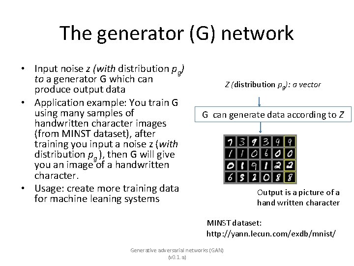
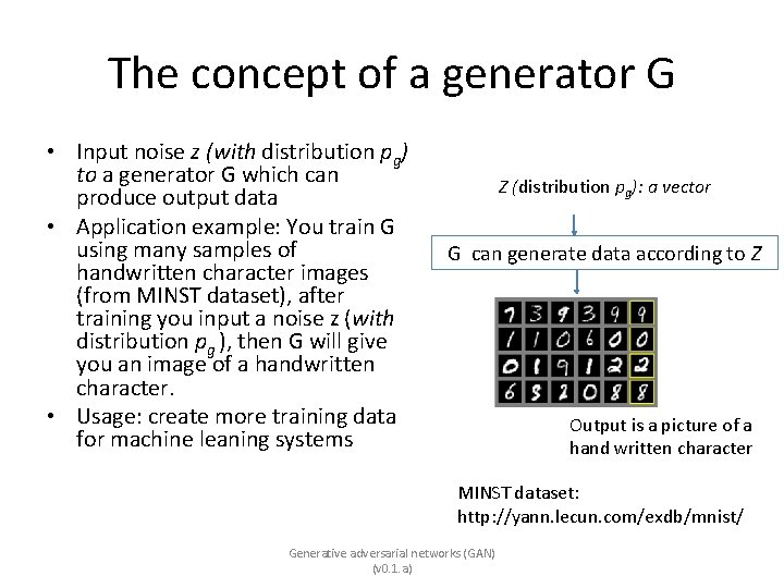
The generator (G) network • Input noise z (with distribution pg) to a generator G which can produce output data • Application example: You train G using many samples of handwritten character images (from MINST dataset), after training you input a noise z (with distribution pg ), then G will give you an image of a handwritten character. • Usage: create more training data for machine leaning systems Z (distribution pg): a vector G can generate data according to Z Output is a picture of a hand written character MINST dataset: http: //yann. lecun. com/exdb/mnist/ Generative adversarial networks (GAN) (v 0. 1. a)

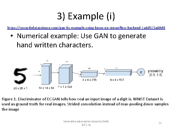
3) Example (i) https: //towardsdatascience. com/gan-by-example-using-keras-on-tensorflow-backend-1 a 6 d 515 a 60 d 0 • Numerical example: Use GAN to generate hand written characters. Figure 1. Discriminator of DCGAN tells how real an input image of a digit is. MNIST Dataset is used as ground truth for real images. Strided convolution instead of max-pooling down samples the image Generative adversarial networks (GAN) (v 0. 1. a) 11

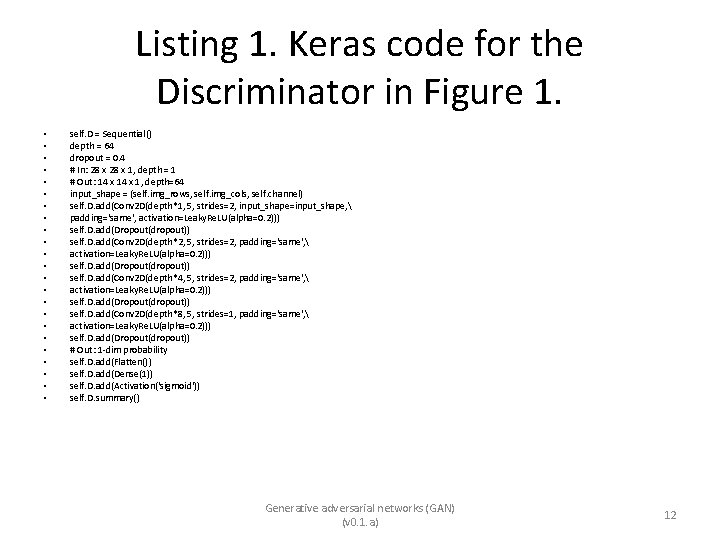
Listing 1. Keras code for the Discriminator in Figure 1. • • • • • • self. D = Sequential() depth = 64 dropout = 0. 4 # In: 28 x 1, depth = 1 # Out: 14 x 1, depth=64 input_shape = (self. img_rows, self. img_cols, self. channel) self. D. add(Conv 2 D(depth*1, 5, strides=2, input_shape=input_shape, padding='same', activation=Leaky. Re. LU(alpha=0. 2))) self. D. add(Dropout(dropout)) self. D. add(Conv 2 D(depth*2, 5, strides=2, padding='same', activation=Leaky. Re. LU(alpha=0. 2))) self. D. add(Dropout(dropout)) self. D. add(Conv 2 D(depth*4, 5, strides=2, padding='same', activation=Leaky. Re. LU(alpha=0. 2))) self. D. add(Dropout(dropout)) self. D. add(Conv 2 D(depth*8, 5, strides=1, padding='same', activation=Leaky. Re. LU(alpha=0. 2))) self. D. add(Dropout(dropout)) # Out: 1 -dim probability self. D. add(Flatten()) self. D. add(Dense(1)) self. D. add(Activation('sigmoid')) self. D. summary() Generative adversarial networks (GAN) (v 0. 1. a) 12

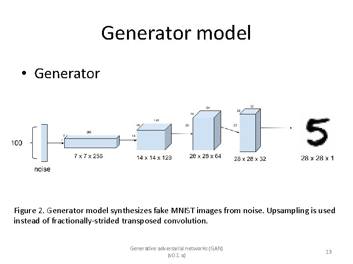
Generator model • Generator Figure 2. Generator model synthesizes fake MNIST images from noise. Upsampling is used instead of fractionally-strided transposed convolution. Generative adversarial networks (GAN) (v 0. 1. a) 13

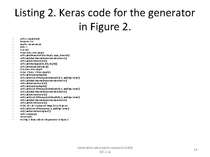
Listing 2. Keras code for the generator in Figure 2. • • • • • • • • self. G = Sequential() dropout = 0. 4 depth = 64+64+64+64 dim = 7 # In: 100 # Out: dim x depth self. G. add(Dense(dim*depth, input_dim=100)) self. G. add(Batch. Normalization(momentum=0. 9)) self. G. add(Activation('relu')) self. G. add(Reshape((dim, depth))) self. G. add(Dropout(dropout)) # In: dim x depth # Out: 2*dim x depth/2 self. G. add(Up. Sampling 2 D()) self. G. add(Conv 2 DTranspose(int(depth/2), 5, padding='same')) self. G. add(Batch. Normalization(momentum=0. 9)) self. G. add(Activation('relu')) self. G. add(Up. Sampling 2 D()) self. G. add(Conv 2 DTranspose(int(depth/4), 5, padding='same')) self. G. add(Batch. Normalization(momentum=0. 9)) self. G. add(Activation('relu')) self. G. add(Conv 2 DTranspose(int(depth/8), 5, padding='same')) self. G. add(Batch. Normalization(momentum=0. 9)) self. G. add(Activation('relu')) # Out: 28 x 1 grayscale image [0. 0, 1. 0] per pix self. G. add(Conv 2 DTranspose(1, 5, padding='same')) self. G. add(Activation('sigmoid')) self. G. summary() return self. G #Listing 2. Keras code for the generator in Figure 2. Generative adversarial networks (GAN) (v 0. 1. a) 14

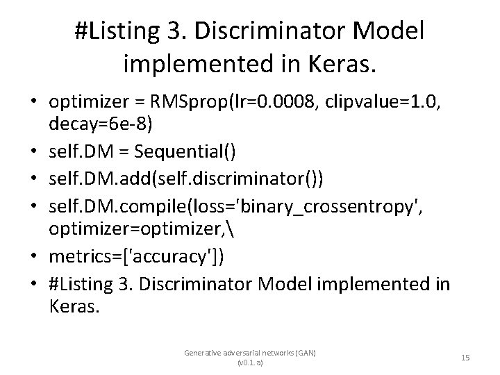
#Listing 3. Discriminator Model implemented in Keras. • optimizer = RMSprop(lr=0. 0008, clipvalue=1. 0, decay=6 e-8) • self. DM = Sequential() • self. DM. add(self. discriminator()) • self. DM. compile(loss='binary_crossentropy', optimizer=optimizer, • metrics=['accuracy']) • #Listing 3. Discriminator Model implemented in Keras. Generative adversarial networks (GAN) (v 0. 1. a) 15

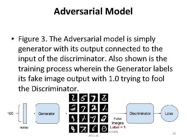
Adversarial Model • Figure 3. The Adversarial model is simply generator with its output connected to the input of the discriminator. Also shown is the training process wherein the Generator labels its fake image output with 1. 0 trying to fool the Discriminator. Generative adversarial networks (GAN) (v 0. 1. a) 16

Listing 4. Adversarial Model as shown in Figure 3 implemented in Keras. • optimizer = RMSprop(lr=0. 0004, clipvalue=1. 0, decay=3 e-8) • self. AM = Sequential() • self. AM. add(self. generator()) • self. AM. add(self. discriminator()) • self. AM. compile(loss='binary_crossentropy', optimizer=optimizer, • metrics=['accuracy']) • #Listing 4. Adversarial Model as shown in Figure 3 implemented in Keras. Generative adversarial networks (GAN) (v 0. 1. a) 17

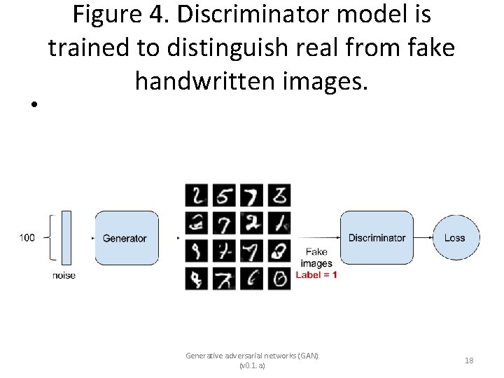
Figure 4. Discriminator model is trained to distinguish real from fake handwritten images. • Generative adversarial networks (GAN) (v 0. 1. a) 18

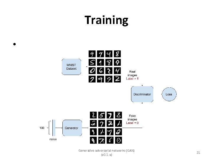
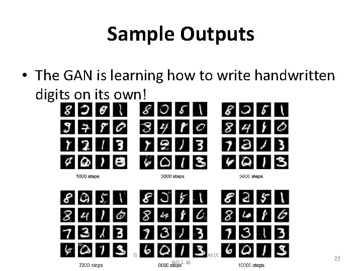
Training • • • images_train = self. x_train[np. random. randint(0, self. x_train. shape[0], size=batch_size), : , : ] noise = np. random. uniform(-1. 0, size=[batch_size, 100]) images_fake = self. generator. predict(noise) x = np. concatenate((images_train, images_fake)) y = np. ones([2*batch_size, 1]) y[batch_size: , : ] = 0 d_loss = self. discriminator. train_on_batch(x, y) y = np. ones([batch_size, 1]) noise = np. random. uniform(-1. 0, size=[batch_size, 100]) a_loss = self. adversarial. train_on_batch(noise, y) #Listing 5. Sequential training of Discriminator Model and Adversarial Model. Training steps above 1000 generates respectable outputs. Generative adversarial networks (GAN) (v 0. 1. a) 19

Training GAN models requires a lot of patience due to its depth. Here are some pointers: • Problem: generated images look like noise. Solution: use dropout on both Discriminator and Generator. Low dropout values (0. 3 to 0. 6) generate more realistic images. • Problem: Discriminator loss converges rapidly to zero thus preventing the Generator from learning. Solution: Do not pre-train the Discriminator. Instead make its learning rate bigger than the Adversarial model learning rate. Use a different training noise sample for the Generator. • Problem: generator images still look like noise. Solution: check if the activation, batch normalization and dropout are applied in the correct sequence. • Problem: figuring out the correct training/model parameters. Solution: start with some known working values from published papers and codes and adjust one parameter at a time. Before training for 2000 or more steps, observe the effect of parameter value adjustment at about 500 or 1000 steps. Generative adversarial networks (GAN) (v 0. 1. a) 20

Training • Generative adversarial networks (GAN) (v 0. 1. a) 21

Sample Outputs • The GAN is learning how to write handwritten digits on its own! Generative adversarial networks (GAN) (v 0. 1. a) 22

Reference • https: //github. com/roatienza/Deep-Learning. Experiments/blob/master/Experiments/Tenso rflow/GAN/dcgan_mnist. py Generative adversarial networks (GAN) (v 0. 1. a) 23

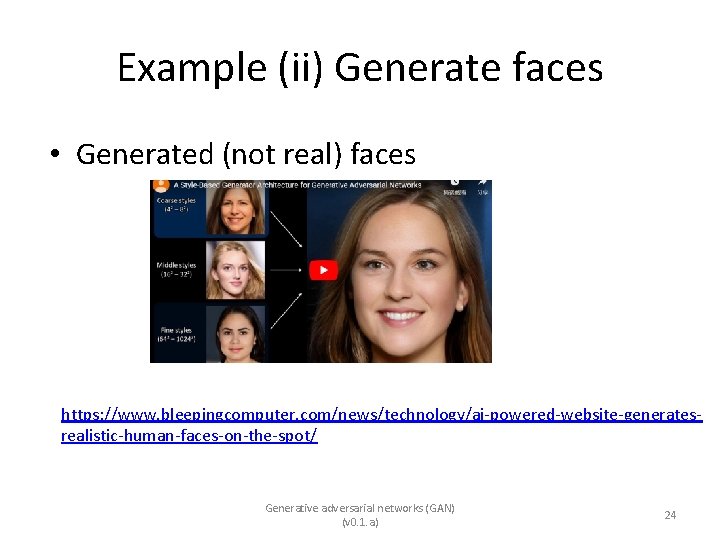
Example (ii) Generate faces • Generated (not real) faces https: //www. bleepingcomputer. com/news/technology/ai-powered-website-generatesrealistic-human-faces-on-the-spot/ Generative adversarial networks (GAN) (v 0. 1. a) 24

4) Case study Edge detection using GAN Generative adversarial networks (GAN) (v 0. 1. a) 25

Generative adversarial networks (GANs) for edge detection Z. Zeng Y. K. Yu, K. H. Wong In IEEE iciev 2018, International Conference on Informatics, Electronics & Vision 'June, kitakyushu exhibition center, japan, 25~29, 2018. (http: //cennser. org/ICIEV/scope-topics. html) Generative adversarial networks (GAN) (v 0. 1. a) 26

Overview • • • Introduction Background Theory Experiment Discussions / Future work Conclusion Generative adversarial networks (GAN) (v 0. 1. a) 27

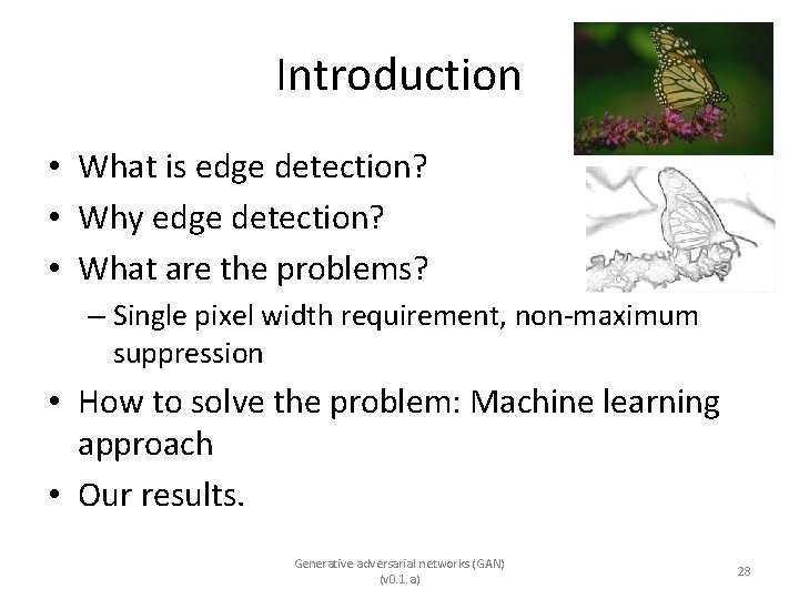
Introduction • What is edge detection? • Why edge detection? • What are the problems? – Single pixel width requirement, non-maximum suppression • How to solve the problem: Machine learning approach • Our results. Generative adversarial networks (GAN) (v 0. 1. a) 28

Background of edge detection • Traditional methods – Sobel, etc. – Canny • Machine learning methods – CNN methods – RCF (state of the art) – Generative adversarial networks (GANs) – Conditional GAN (c. GANs) – c. GAN with U-NET (=our approach, first team to apply c. GAN for edge detection) https: //lmb. informatik. uni-freiburg. de/people/ronneber/u-net/ Generative adversarial networks (GAN) (v 0. 1. a) 29

Theory of Generative adversarial networks (GAN) • GAN • Discriminator (D) • Generator(G) Generative adversarial networks (GAN) (v 0. 1. a) 30

Application of GAN • Generate data with the same distribution of training samples • Application : Enrich data sets, e. g. use some data in MINST dataset to train G, so G can generate more training samples. • Good for face datasets etc. MINST dataset: http: //yann. lecun. com/exdb/mnist/ Generative adversarial networks (GAN) (v 0. 1. a) 31

The idea, from : Goodfellow, Ian, et al. "Generative adversarial nets. " Advances in neural information processing systems. 2014. https: //arxiv. org/abs/1406. 2661 • The proposed adversarial nets framework, the generative model is pitted against an adversary: • a discriminative model (D) that learns to determine whether a sample is from the model distribution or the data distribution. The generative model (G) can be thought of as analogous to a team of counterfeiters, trying to produce fake currency and use it without detection, while the discriminative model is analogous to the police, trying to detect the counterfeit currency. Competition in this game drives both teams to improve their methods until the counterfeits are indistinguishable from the genuine articles. Generative adversarial networks (GAN) (v 0. 1. a) 32

The concept of a generator G • Input noise z (with distribution pg) to a generator G which can produce output data • Application example: You train G using many samples of handwritten character images (from MINST dataset), after training you input a noise z (with distribution pg ), then G will give you an image of a handwritten character. • Usage: create more training data for machine leaning systems Z (distribution pg): a vector G can generate data according to Z Output is a picture of a hand written character MINST dataset: http: //yann. lecun. com/exdb/mnist/ Generative adversarial networks (GAN) (v 0. 1. a)

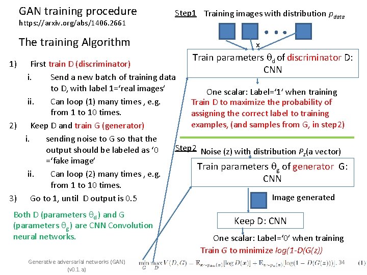
GAN training procedure https: //arxiv. org/abs/1406. 2661 The training Algorithm Step 1 Training images with distribution pdata x Train parameters of discriminator D: d First train D (discriminator) CNN i. Send a new batch of training data to D, with label 1=‘real images’ One scalar: Label=‘ 1’ when training ii. Can loop (1) many times , e. g. Train D to maximize the probability of from 1 to 10 times. assigning the correct label to training examples, (and samples from G, in step 2) 2) Keep D and train G (generator) i. sending noise to G so that the Step 2 Noise (z) with distribution P (a vector) output should be labeled as ‘ 0 z =‘fake image’ Train parameters g of generator G: ii. Can loop (2) many times , e. g. CNN from 1 to 10 times. Image generated 3) Go to 1, until D output is 0. 5 1) Both D (parameters d ) and G (parameters g ) are CNN Convolution neural networks. Generative adversarial networks (GAN) (v 0. 1. a) Keep D: CNN One scalar: Label=‘ 0’ when training Train G to minimize log(1 -D(G(z)) 34

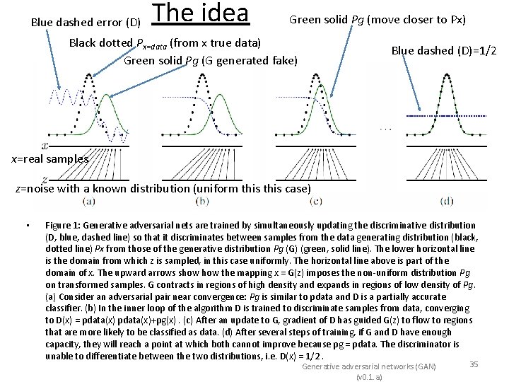
The idea Blue dashed error (D) Green solid Pg (move closer to Px) Black dotted Px=data (from x true data) Green solid Pg (G generated fake) Blue dashed (D)=1/2 x=real samples z=noise with a known distribution (uniform this case) • Figure 1: Generative adversarial nets are trained by simultaneously updating the discriminative distribution (D, blue, dashed line) so that it discriminates between samples from the data generating distribution (black, dotted line) Px from those of the generative distribution Pg (G) (green, solid line). The lower horizontal line is the domain from which z is sampled, in this case uniformly. The horizontal line above is part of the domain of x. The upward arrows show the mapping x = G(z) imposes the non-uniform distribution Pg on transformed samples. G contracts in regions of high density and expands in regions of low density of Pg. (a) Consider an adversarial pair near convergence: Pg is similar to pdata and D is a partially accurate classifier. (b) In the inner loop of the algorithm D is trained to discriminate samples from data, converging to D(x) = pdata(x)+pg(x). (c) After an update to G, gradient of D has guided G(z) to flow to regions that are more likely to be classified as data. (d) After several steps of training, if G and D have enough capacity, they will reach a point at which both cannot improve because pg = pdata. The discriminator is unable to differentiate between the two distributions, i. e. D(x) = 1/2. Generative adversarial networks (GAN) (v 0. 1. a) 35

c. GAN (conditional GAN ) GAN is difficult to train when the search space is too large. Use c. GAN Generative adversarial networks (GAN) (v 0. 1. a) 36

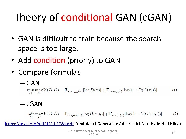
Theory of conditional GAN (c. GAN) • GAN is difficult to train because the search space is too large. • Add condition (prior y) to GAN • Compare formulas – GAN – c. GAN https: //arxiv. org/pdf/1411. 1784. pdf Conditional Generative Adversarial Nets by Mehdi Mirza Generative adversarial networks (GAN) (v 0. 1. a) 37

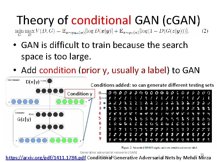
Theory of conditional GAN (c. GAN) • GAN is difficult to train because the search space is too large. • Add condition (prior y, usually a label) to GAN D(x|y) Conditions added: so can generate different testing sets Condition y G(z|y) 0 1 2 3 4 5 6 7 8 9 Generative adversarial networks (GAN) 38 (v 0. 1. a) https: //arxiv. org/pdf/1411. 1784. pdf Conditional Generative Adversarial Nets by Mehdi Mirza

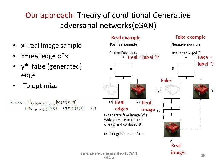
Our approach: Theory of conditional Generative adversarial networks(c. GAN) Fake example Real example • x=real image sample • Y=real edge of x • y*=false (generated) edge • To optimize Real = label ‘ 1’ Fake = label ‘ 0’ Fake Real edges Generative adversarial networks (GAN) (v 0. 1. a) Real image 39

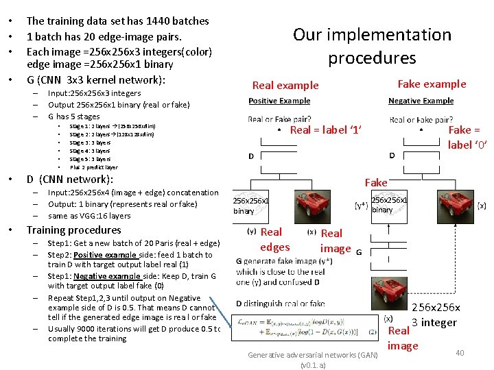
• • The training data set has 1440 batches 1 batch has 20 edge-image pairs. Each image =256 x 3 integers(color) edge image =256 x 1 binary G (CNN 3 x 3 kernel network): – – – Input: 256 x 3 integers Output 256 x 1 binary (real or fake) G has 5 stages • • Fake example Real = label ‘ 1’ Stage 1: 2 layers (256 xdim) Stage 2: 2 layers (128 xdim) Stage 3: 3 layers Stage 4: 3 layers Stage 5: 3 layers Plus 2 predict layer D (CNN network): – – – • Our implementation procedures Input: 256 x 4 (image + edge) concatenation Output: 1 binary (represents real or fake) same as VGG: 16 layers Training procedures – – – Step 1: Get a new batch of 20 Paris (real + edge) Step 2: Positive example side: feed 1 batch to train D with target output label real (1) Step 1: Negative example side: Keep D, train G with target output label fake (0) Repeat Step 1, 2, 3 until output on Negative example side of D is 0. 5. That means D cannot tell if the generated edge image is rea l or fake Usually 9000 iterations will get D produce 0. 5 to complete the training Fake = label ‘ 0’ Fake 256 x 1 binary Real edges Real image Generative adversarial networks (GAN) (v 0. 1. a) 256 x 3 integer Real image 40

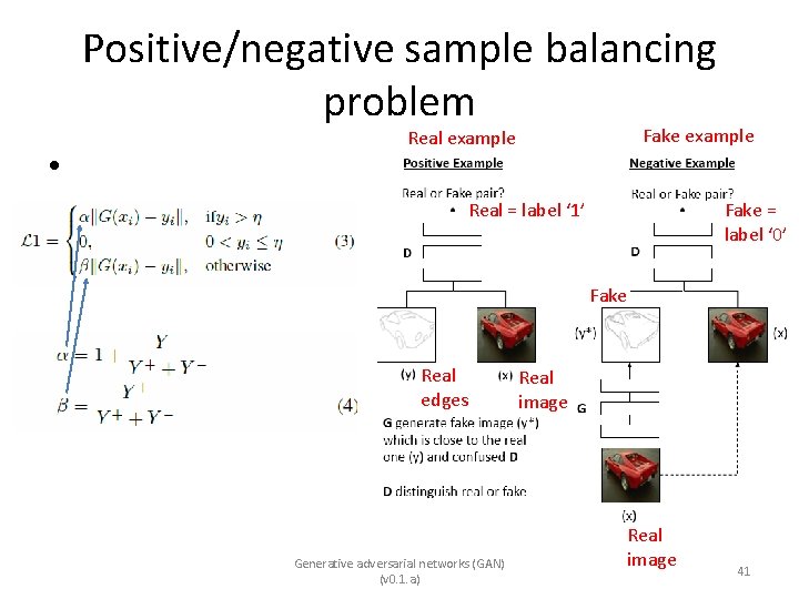
Positive/negative sample balancing problem • Fake example Real = label ‘ 1’ Fake = label ‘ 0’ Fake Real edges Generative adversarial networks (GAN) (v 0. 1. a) Real image 41

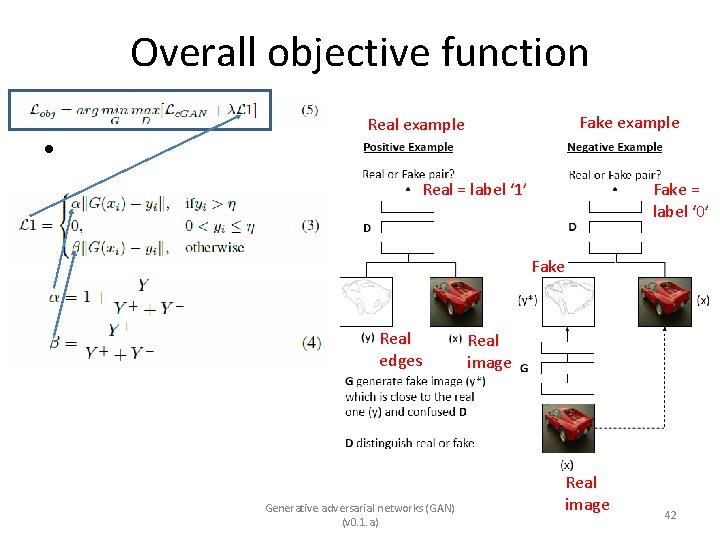
Overall objective function • Fake example Real = label ‘ 1’ Fake = label ‘ 0’ Fake Real edges Generative adversarial networks (GAN) (v 0. 1. a) Real image 42

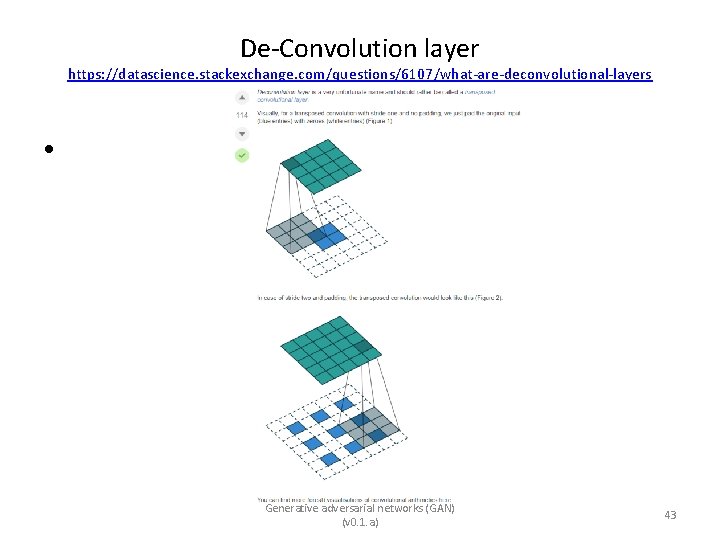
De-Convolution layer https: //datascience. stackexchange. com/questions/6107/what-are-deconvolutional-layers • Generative adversarial networks (GAN) (v 0. 1. a) 43

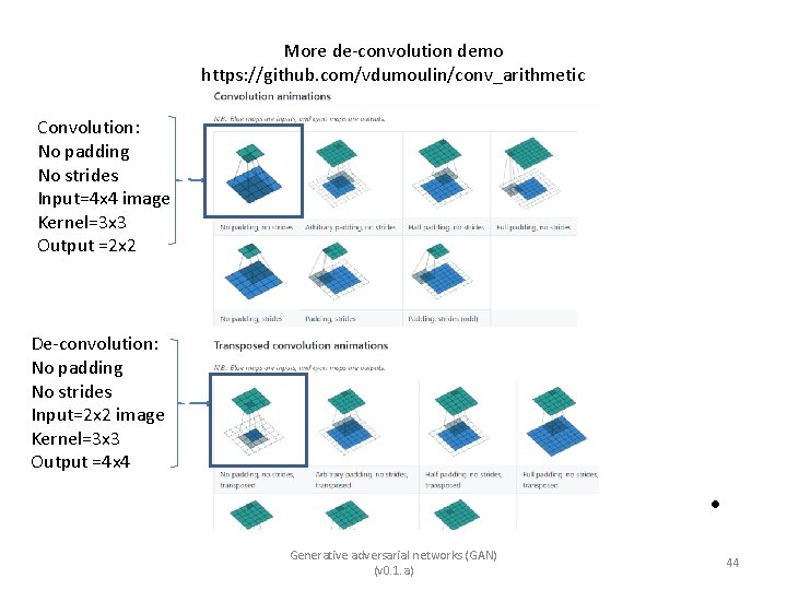
More de-convolution demo https: //github. com/vdumoulin/conv_arithmetic Convolution: No padding No strides Input=4 x 4 image Kernel=3 x 3 Output =2 x 2 De-convolution: No padding No strides Input=2 x 2 image Kernel=3 x 3 Output =4 x 4 • Generative adversarial networks (GAN) (v 0. 1. a) 44

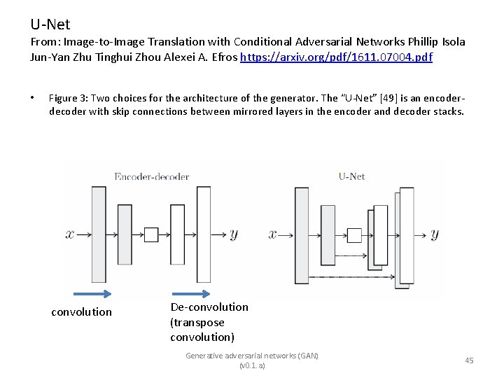
U-Net From: Image-to-Image Translation with Conditional Adversarial Networks Phillip Isola Jun-Yan Zhu Tinghui Zhou Alexei A. Efros https: //arxiv. org/pdf/1611. 07004. pdf • Figure 3: Two choices for the architecture of the generator. The “U-Net” [49] is an encoderdecoder with skip connections between mirrored layers in the encoder and decoder stacks. convolution De-convolution (transpose convolution) Generative adversarial networks (GAN) (v 0. 1. a) 45

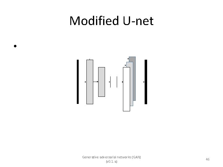
Modified U-net • Generative adversarial networks (GAN) (v 0. 1. a) 46

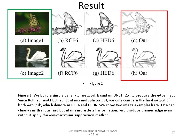
Result • • Figure 1. We build a simple generator network based on UNET [25] to produce the edge map. Since RCF [23] and HED [28] contains multiple output, we only compare the final output of both network, which denote as RCF 6 and HED 6. We show two image examples here. One can clearly see that our result contains more detail information, and produce thinner edge even without apply the non-maximum suppression method. Generative adversarial networks (GAN) (v 0. 1. a) 47

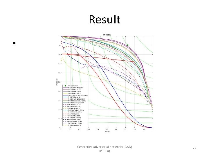
Result • Generative adversarial networks (GAN) (v 0. 1. a) 48

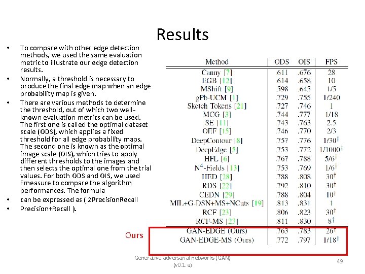
• • • To compare with other edge detection methods, we used the same evaluation metric to illustrate our edge detection results. Normally, a threshold is necessary to produce the final edge map when an edge probability map is given. There are various methods to determine threshold, out of which two wellknown evaluation metrics can be used. The first one is called the optimal dataset scale (ODS), which applies a fixed threshold for all edge probability maps. The second one is known as the optimal image scale (OIS), which tries to apply different thresholds to the images and then selects the optimal one from the trial values. For both ODS and OIS, we used Fmeasure to compare the algorithm performances. The formula can be expressed as ( 2 Precision. Recall Precision+Recall ). Results Ours Generative adversarial networks (GAN) (v 0. 1. a) 49

Discussions/ Future work • Generative adversarial networks (GAN) (v 0. 1. a) 50

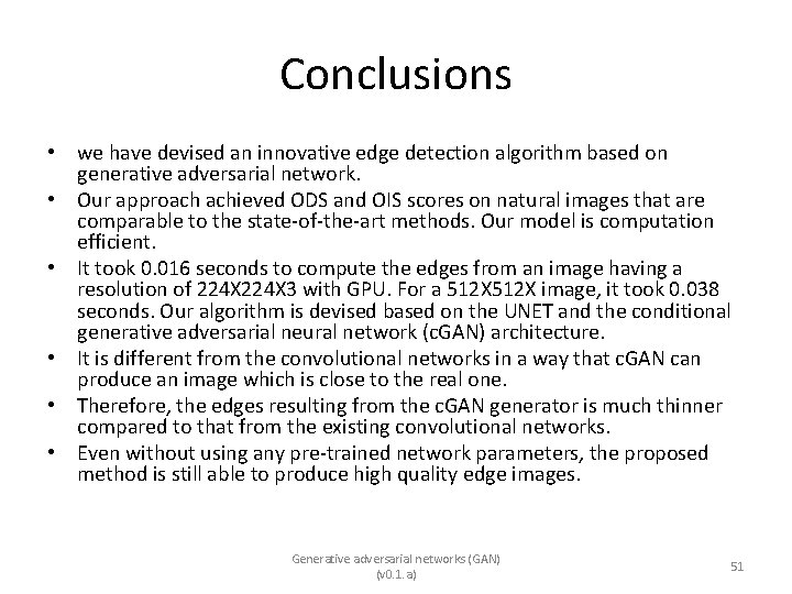
Conclusions • we have devised an innovative edge detection algorithm based on generative adversarial network. • Our approach achieved ODS and OIS scores on natural images that are comparable to the state-of-the-art methods. Our model is computation efficient. • It took 0. 016 seconds to compute the edges from an image having a resolution of 224 X 3 with GPU. For a 512 X image, it took 0. 038 seconds. Our algorithm is devised based on the UNET and the conditional generative adversarial neural network (c. GAN) architecture. • It is different from the convolutional networks in a way that c. GAN can produce an image which is close to the real one. • Therefore, the edges resulting from the c. GAN generator is much thinner compared to that from the existing convolutional networks. • Even without using any pre-trained network parameters, the proposed method is still able to produce high quality edge images. Generative adversarial networks (GAN) (v 0. 1. a) 51