Generative Adversarial Imitation Learning Stefano Ermon Joint work

Generative Adversarial Imitation Learning Stefano Ermon Joint work with Jayesh Gupta, Jonathan Ho, Yunzhu Li, and Jiaming Song

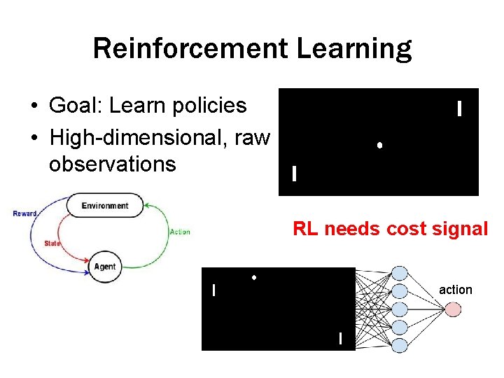
Reinforcement Learning • Goal: Learn policies • High-dimensional, raw observations RL needs cost signal action

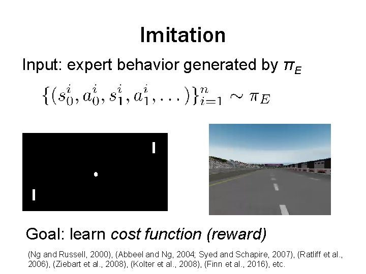
Imitation Input: expert behavior generated by πE Goal: learn cost function (reward) (Ng and Russell, 2000), (Abbeel and Ng, 2004; Syed and Schapire, 2007), (Ratliff et al. , 2006), (Ziebart et al. , 2008), (Kolter et al. , 2008), (Finn et al. , 2016), etc.

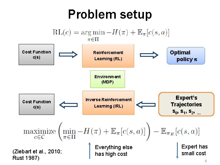
Problem setup Cost Function c(s) Reinforcement Learning (RL) Optimal policy p Environment (MDP) Cost Function c(s) (Ziebart et al. , 2010; Rust 1987) Inverse Reinforcement Learning (IRL) Everything else has high cost Expert’s Trajectories s 0 , s 1 , s 2 , … Expert has small cost 4

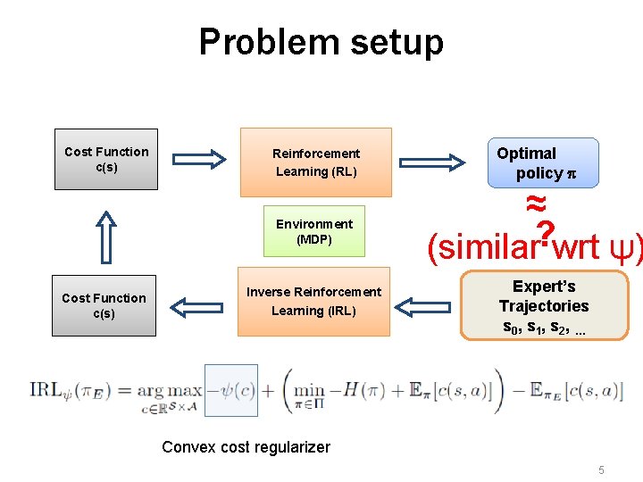
Problem setup Cost Function c(s) Reinforcement Learning (RL) Environment (MDP) Cost Function c(s) Inverse Reinforcement Learning (IRL) Optimal policy p ≈ ? (similar wrt ψ) Expert’s Trajectories s 0 , s 1 , s 2 , … Convex cost regularizer 5

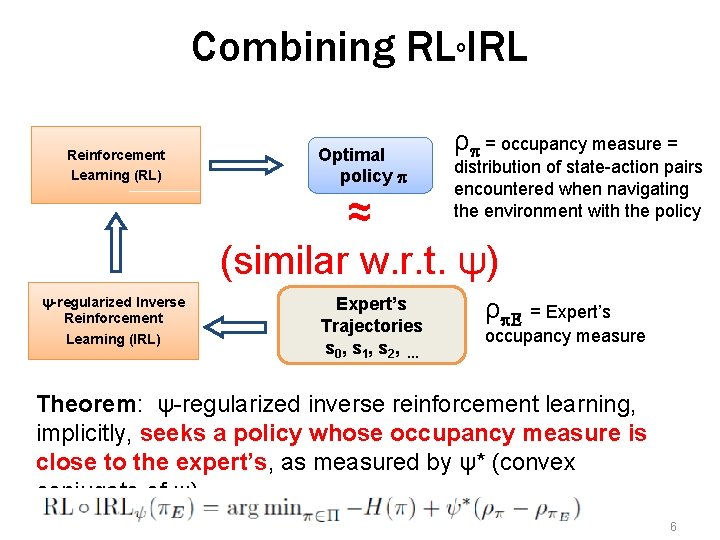
Combining RLo. IRL Reinforcement Learning (RL) Optimal policy p ρp = occupancy measure = distribution of state-action pairs encountered when navigating the environment with the policy ≈ (similar w. r. t. ψ) ψ-regularized Inverse Reinforcement Learning (IRL) Expert’s Trajectories s 0 , s 1 , s 2 , … ρp. E = Expert’s occupancy measure Theorem: ψ-regularized inverse reinforcement learning, implicitly, seeks a policy whose occupancy measure is close to the expert’s, as measured by ψ* (convex conjugate of ψ) 6

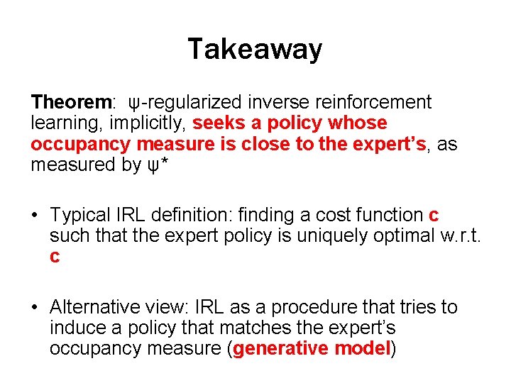
Takeaway Theorem: ψ-regularized inverse reinforcement learning, implicitly, seeks a policy whose occupancy measure is close to the expert’s, as measured by ψ* • Typical IRL definition: finding a cost function c such that the expert policy is uniquely optimal w. r. t. c • Alternative view: IRL as a procedure that tries to induce a policy that matches the expert’s occupancy measure (generative model)

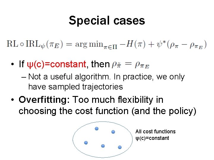
Special cases • If ψ(c)=constant, then – Not a useful algorithm. In practice, we only have sampled trajectories • Overfitting: Too much flexibility in choosing the cost function (and the policy) All cost functions ψ(c)=constant

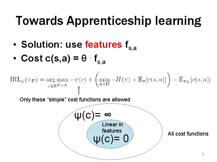
Towards Apprenticeship learning • Solution: use features fs, a • Cost c(s, a) = θ. fs, a Only these “simple” cost functions are allowed ψ(c)= ∞ Linear in features ψ(c)= 0 All cost functions 9

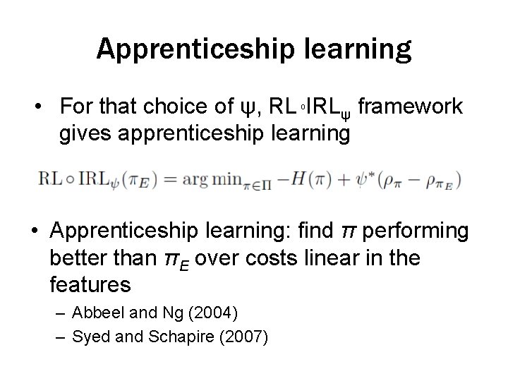
Apprenticeship learning • For that choice of ψ, RL IRLψ framework gives apprenticeship learning o • Apprenticeship learning: find π performing better than πE over costs linear in the features – Abbeel and Ng (2004) – Syed and Schapire (2007)

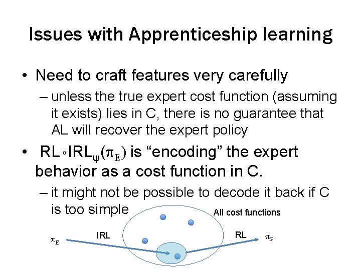
Issues with Apprenticeship learning • Need to craft features very carefully – unless the true expert cost function (assuming it exists) lies in C, there is no guarantee that AL will recover the expert policy • RL IRLψ(p. E) is “encoding” the expert behavior as a cost function in C. o – it might not be possible to decode it back if C is too simple All cost functions p. E IRL RL p. R

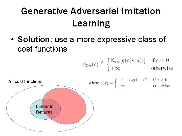
Generative Adversarial Imitation Learning • Solution: use a more expressive class of cost functions All cost functions Linear in features

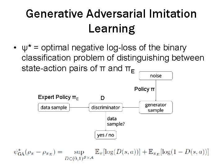
Generative Adversarial Imitation Learning • ψ* = optimal negative log-loss of the binary classification problem of distinguishing between state-action pairs of π and πE Policy π Expert Policy πE D

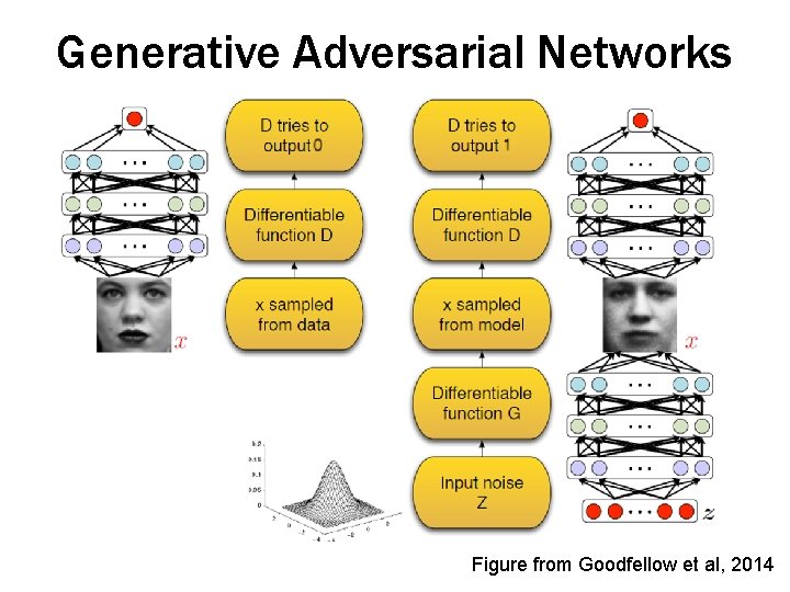
Generative Adversarial Networks Figure from Goodfellow et al, 2014

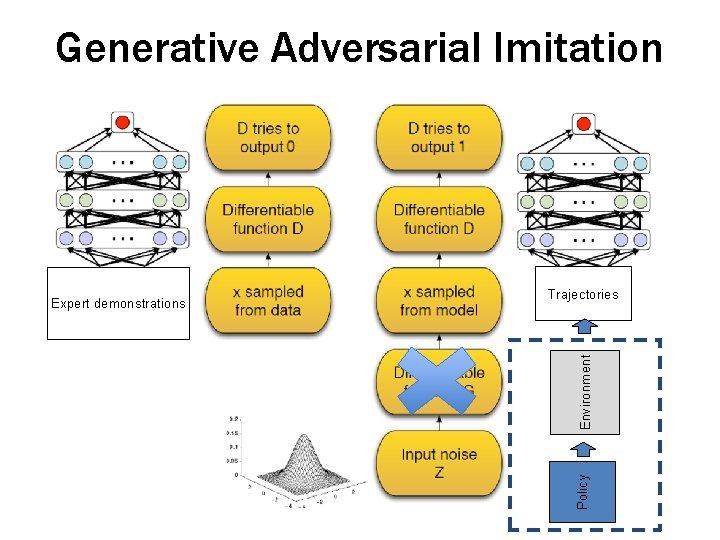
Generative Adversarial Imitation Environment Trajectories Policy Expert demonstrations

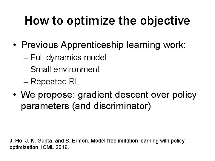
How to optimize the objective • Previous Apprenticeship learning work: – Full dynamics model – Small environment – Repeated RL • We propose: gradient descent over policy parameters (and discriminator) J. Ho, J. K. Gupta, and S. Ermon. Model-free imitation learning with policy optimization. ICML 2016.

Properties • Inherits pros of policy gradient – Convergence to local minima – Can be model free • Inherits cons of policy gradient – High variance – Small steps required

Properties • Inherits pros of policy gradient – Convergence to local minima – Can be model free • Inherits cons of policy gradient – High variance – Small steps required • Solution: trust region policy optimization

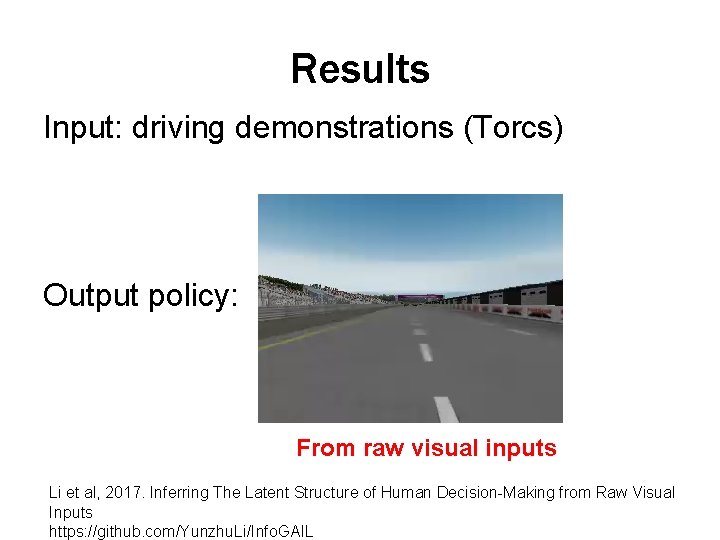
Results Input: driving demonstrations (Torcs) Output policy: From raw visual inputs Li et al, 2017. Inferring The Latent Structure of Human Decision-Making from Raw Visual Inputs https: //github. com/Yunzhu. Li/Info. GAIL

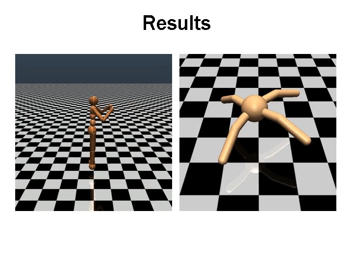
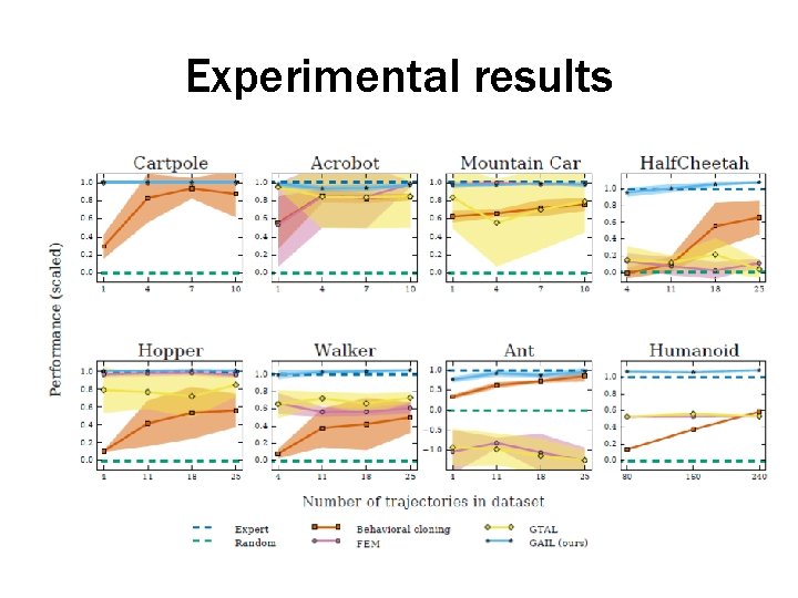
Results

Experimental results

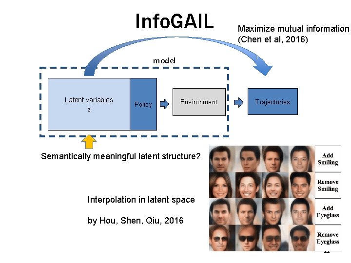
Info. GAIL Maximize mutual information (Chen et al, 2016) model Latent variables Z Policy Environment Trajectories Semantically meaningful latent structure? Interpolation in latent space by Hou, Shen, Qiu, 2016 22

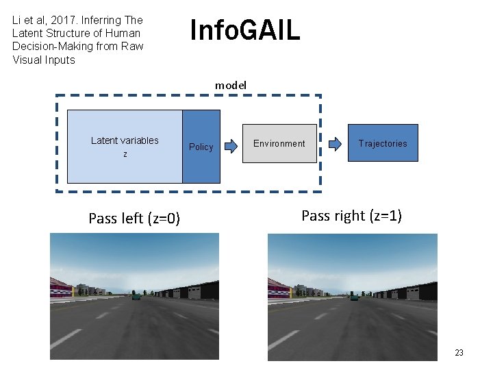
Li et al, 2017. Inferring The Latent Structure of Human Decision-Making from Raw Visual Inputs Info. GAIL model Latent variables Z Pass left (z=0) Policy Environment Trajectories Pass right (z=1) 23

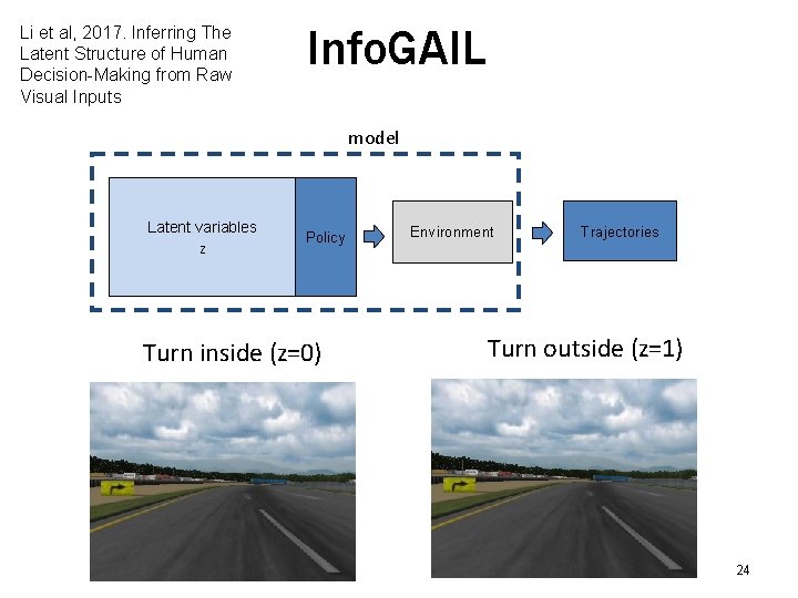
Li et al, 2017. Inferring The Latent Structure of Human Decision-Making from Raw Visual Inputs Info. GAIL model Latent variables Z Policy Turn inside (z=0) Environment Trajectories Turn outside (z=1) 24

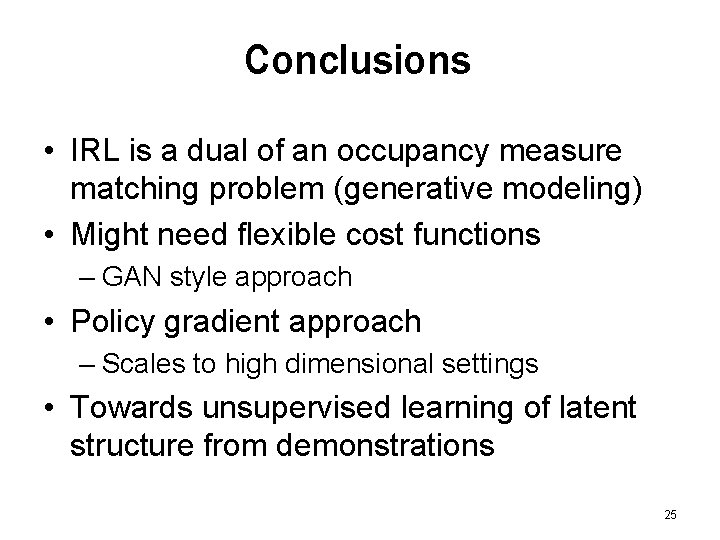
Conclusions • IRL is a dual of an occupancy measure matching problem (generative modeling) • Might need flexible cost functions – GAN style approach • Policy gradient approach – Scales to high dimensional settings • Towards unsupervised learning of latent structure from demonstrations 25