Generation of PPM Detection Of PPM Pulse Code

Generation of PPM

Detection Of PPM

Pulse Code Modulation (PCM) 3

PCM Volts 8 8 5 -1 -2 -9 time -7 01000 10010 11001 10001 00101 10111 4 time

Merits of Digital Communication: 1. Digital signals are very easy to receive. The receiver has to just detect whether the pulse is low or high. 2. AM & FM signals become corrupted over much short distances as compared to digital signals. In digital signals, the original signal can be reproduced accurately. 3. The signals lose power as they travel, which is called attenuation. When AM and FM signals are amplified, the noise also get amplified. But the digital signals can be cleaned up to restore the quality and amplified by the regenerators. 4. The noise may change the shape of the pulses but not the pattern of the pulses. 5. AM and FM signals can be received by any one by suitable receiver. But digital signals can be coded so that only the person, who is intended for, can receive them. 6. 5 The digital signals can be stored, or used to produce a display on a computer monitor or converted back into analog signal to drive a loud speaker.

Error correction Easy processing and storage Disadvantages: More bandwidth Need of ADC and DAC Need of clock recovery circuit Incompatible with older analog system 6

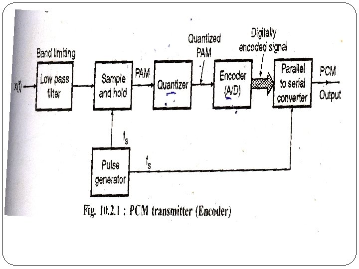
Pulse Code Modulation (PCM): • Analog signal is converted into digital signal by using a digital code. Analog to digital converter employs two techniques: 1. Sampling: The process of generating pulses of zero width and of amplitude equal to the instantaneous amplitude of the analog signal. The no. of pulses per second is called “sampling rate”. 2. Quantization: The process of dividing the maximum value of the analog signal into a fixed no. of levels in order to convert the PAM into a Binary Code. The levels obtained are called “quanization levels”. * A digital signal is described by its ‘bit rate’ whereas analog signal is described by its ‘frequency range’. * 7 Bit rate = sampling rate x no. of bits / sample

Sampling, Quantization and Coding V o l t a g e Time L e v e ls 111 110 101 100 011 010 001 000 7 6 5 4 3 2 1 0 V o l t a g e B i n a r y Time 0 1 01 01 1 1 1 1 0 10 1 0 Time C o d e s

Quantization § Is the process of converting the sampled signal to a binary value § Each voltage level will correspond to a different binary number § The magnitude of the minimum step size is called the resolution. § Resolution with respect to digitizing system refers to the accuracy of the digitizing system in representing the sampled signal. § The error resulting from quantizing is called the quantization noise. Its value is 1/2 the resolution

1. Sampling ( Time axis) 2. Quantization (Amplitude axis) 3. encoding 111 110 101 100 011 010 001 000 t 0 Encode 011 t 1 101 t 2 110 t 3 101 011 t 4 011 t 5 000 t 7 t 6 001 011 t 8

Quantization example amplitude x(t) 111 3. 1867 110 2. 2762 101 1. 3657 100 0. 4552 Step size Quant. levels boundaries 011 -0. 4552 010 -1. 3657 001 -2. 2762 xq(n. Ts): quantized values x(n. Ts): sampled values 000 -3. 1867 Ts: sampling time PCM codeword t 110 111 110 100 011 PCM sequence

12

13

14

Quantization Noise 20 levels Red = magnitude Black = timing interval

4 levels Red = magnitude Black = timing interval

Quantization error § Quantizing error: The difference between the input and output of a quantizer Process of quantizing noise Model of quantizing noise Qauntizer AGC + § Maximum quantization error is § Signal to Quantization noise ratio

Dynamic Range This is the ratio of the largest to smallest analogue signal that can be transmitted. But Vmin is the resolution and can be written as It follows that

Types of Quantization 1. Uniform quantizer: if the step size remains constant throughout the input range. There are two types of quantizer: Ø Symmetric quantizer of the mid tread type Ø Symmetric quantizer of the mid riser type. 2. Non uniform quantizer: if the quantizer characteristics is nonlinear and the step size is not constant instead it varies depending on the amplitude of input.

Mid riser 20 Mid trader

Uniform and nonuniform quantization 21

Non-uniform quantization § It is achieved by uniformly quantizing the “compressed” signal. § At the receiver, an inverse compression characteristic, called “expansion” is employed to avoid signal distortion. compression+expansion Compress companding Qauntize Transmitter Expand Channel Receiver

Companding characteristics 23

24

Block Diagram of Companding Process 25

Laws of companding § The µ-law algorithm is a companding algorithm, primarily used in the digital telecommunication systems of North America and Japan. § Companding algorithms reduce the dynamic range of an audio signal. § In analog systems, this can increase the signal-to-noise ratio (SNR) achieved during transmission, and in the digital domain, it can reduce the quantization error (hence increasing signal to quantization noise ratio). 26

Laws of companding An A-law algorithm is a standard companding algorithm, used in European digital communications systems to optimize, i. e. , modify, the dynamic range of an analog signal for digitizing. 27

PCM Receiver

DIFFERENTIAL PCM ØOnly transmit the difference between the predicated value and the actual value ØVoice changes relatively slowly ØIt is possible to predict the value of the simplest form

DPCM TRANSMITTER 31

DPCM Receiver

Delta Modulation § PCM is powerful, but quite complex coders and decoders are required. § An increase in resolution also requires a higher number of bits per sample. § An alternative, which overcomes some limitations of PCM is to use past information in the encoding process. One way of doing this is to perform source coding using delta modulation: § Transmits information only to indicate whether the sample of analog signal is larger or smaller then the previous sample. 33

Principle of DM 34

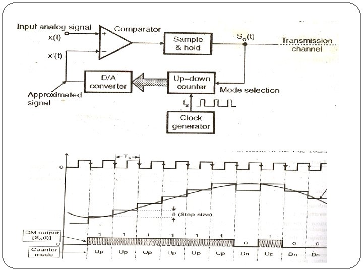
Delta modulation components 35

Types of error 1. Slope overload : happens when analog signal changes at a faster rate than the DAC can maintain. Øincreasing the clock frequency reduces the probability of slope overload occurring. ØAnother way to prevent is to increase the magnitude of step size 37

Types of error 2. Granular noise: when original analog signal has relatively constant amplitude, the reconstructed signal has variations that were not present in the original signal. this is called as granular noise. Ø Can be reduced by decreasing the step size 38

§ To reduce the granular noise, a small resolution(small step size) is needed and to reduce slope overload occurring , a large resolution is required. 39

DM RECEIVER

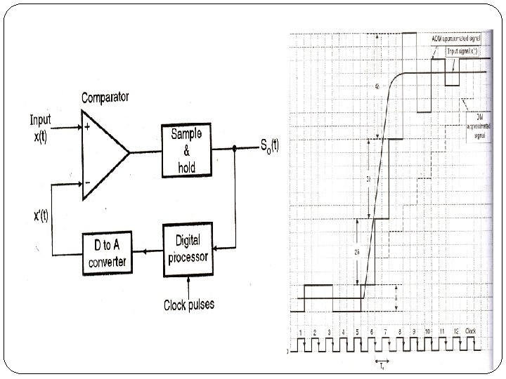
Adaptive Delta Modulation § Is a delta modulation system where the step size of the DAC is varied , depending upon the amplitude characteristics of the analog input signal. § A common algorithm for adaptive delta modulator is when three consecutive 1 s or 0 s occur, the step size of the DAC is increased or decreased by a factor of 1. 5. 41

43