Generating Random Numbers By Dr Jason Merrick What

Generating Random Numbers By Dr. Jason Merrick

What We’ll Do. . . • • Random-number generation Generating random variates Non-stationary Poisson processes Variance reduction 2

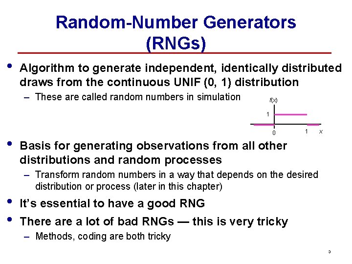
Random-Number Generators (RNGs) • Algorithm to generate independent, identically distributed draws from the continuous UNIF (0, 1) distribution – These are called random numbers in simulation f(x) 1 • • • 0 1 x Basis for generating observations from all other distributions and random processes – Transform random numbers in a way that depends on the desired distribution or process (later in this chapter) It’s essential to have a good RNG There a lot of bad RNGs — this is very tricky – Methods, coding are both tricky 3

Pseudo Random Numbers • • Random numbers generated by a computer are not really random They just behave like random numbers For a large enough sample, the generated values will pass all tests for a uniform distribution – If you look at a histogram of a large number, it will look uniform – Pass chi-square test – Pass Kolmogorov-Smirnov Test The stream of random numbers will pass all the tests for randomness – Runs test – Autocorrelation test Simulation with Arena — Further Statistical Issues 4

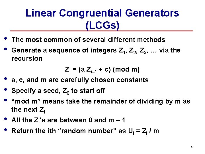
Linear Congruential Generators (LCGs) • • The most common of several different methods Generate a sequence of integers Z 1, Z 2, Z 3, … via the recursion Zi = (a Zi– 1 + c) (mod m) • • • a, c, and m are carefully chosen constants • • All the Zi’s are between 0 and m – 1 Specify a seed, Z 0 to start off “mod m” means take the remainder of dividing by m as the next Zi Return the ith “random number” as Ui = Zi / m 5

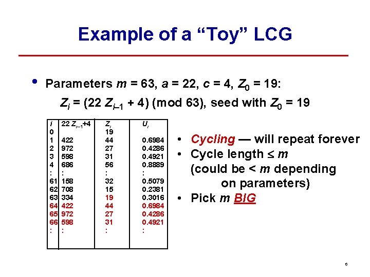
Example of a “Toy” LCG • Parameters m = 63, a = 22, c = 4, Z 0 = 19: Zi = (22 Zi– 1 + 4) (mod 63), seed with Z 0 = 19 i 0 1 2 3 4 : 61 62 63 64 65 66 : 22 Zi– 1+4 422 972 598 686 : 158 708 334 422 972 598 : Zi 19 44 27 31 56 : 32 15 19 44 27 31 : Ui 0. 6984 0. 4286 0. 4921 0. 8889 : 0. 5079 0. 2381 0. 3016 0. 6984 0. 4286 0. 4921 : • Cycling — will repeat forever • Cycle length £ m (could be < m depending on parameters) • Pick m BIG 6

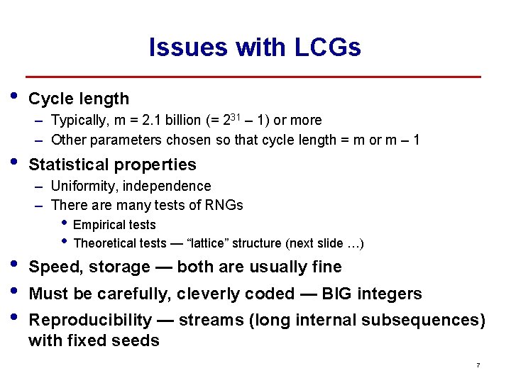
Issues with LCGs • • Cycle length – Typically, m = 2. 1 billion (= 231 – 1) or more – Other parameters chosen so that cycle length = m or m – 1 Statistical properties – Uniformity, independence – There are many tests of RNGs • • • Empirical tests Theoretical tests — “lattice” structure (next slide …) Speed, storage — both are usually fine Must be carefully, cleverly coded — BIG integers Reproducibility — streams (long internal subsequences) with fixed seeds 7

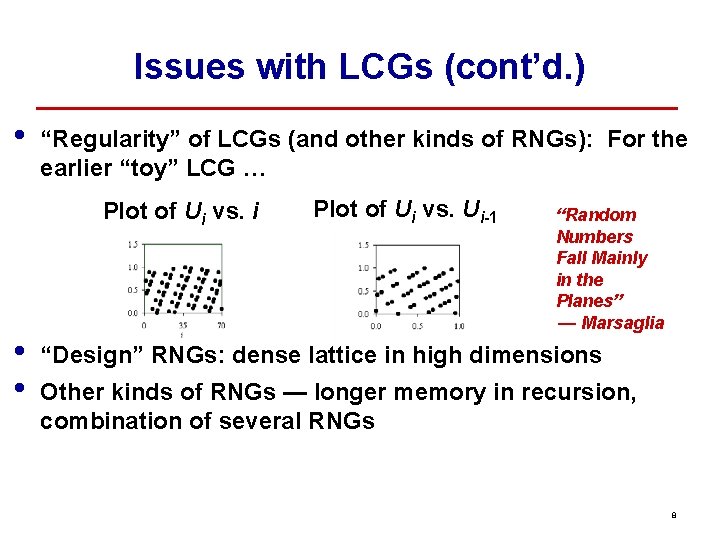
Issues with LCGs (cont’d. ) • “Regularity” of LCGs (and other kinds of RNGs): For the earlier “toy” LCG … Plot of Ui vs. i • • Plot of Ui vs. Ui-1 “Random Numbers Fall Mainly in the Planes” — Marsaglia “Design” RNGs: dense lattice in high dimensions Other kinds of RNGs — longer memory in recursion, combination of several RNGs 8

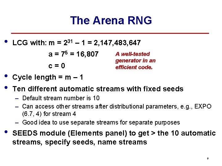
The Arena RNG • LCG with: m = 231 – 1 = 2, 147, 483, 647 a = 75 = 16, 807 • • • c=0 A well-tested generator in an efficient code. Cycle length = m – 1 Ten different automatic streams with fixed seeds – Default stream number is 10 – Can access other streams after distributional parameters, e. g. , EXPO (6. 7, 4) for stream 4 – Good idea to use separate streams for separate purposes SEEDS module (Elements panel) to get > the 10 automatic streams, specify seeds, name streams 9

Generating Random Variates • • Have: Desired input distribution for model (fitted or specified in some way), and RNG (UNIF (0, 1)) Want: Transform UNIF (0, 1) random numbers into “draws” from the desired input distribution Method: Mathematical transformations of random numbers to “deform” them to the desired distribution – Specific transform depends on desired distribution – Details in online Help about methods for all distributions Do discrete, continuous distributions separately 10

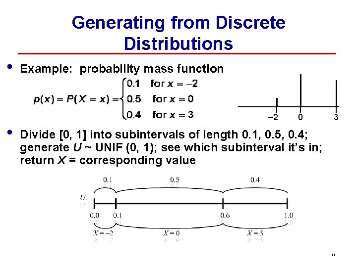
Generating from Discrete Distributions • Example: probability mass function – 2 • 0 3 Divide [0, 1] into subintervals of length 0. 1, 0. 5, 0. 4; generate U ~ UNIF (0, 1); see which subinterval it’s in; return X = corresponding value 11

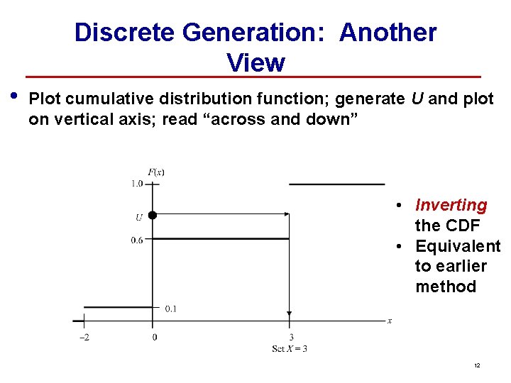
Discrete Generation: Another View • Plot cumulative distribution function; generate U and plot on vertical axis; read “across and down” • Inverting the CDF • Equivalent to earlier method 12

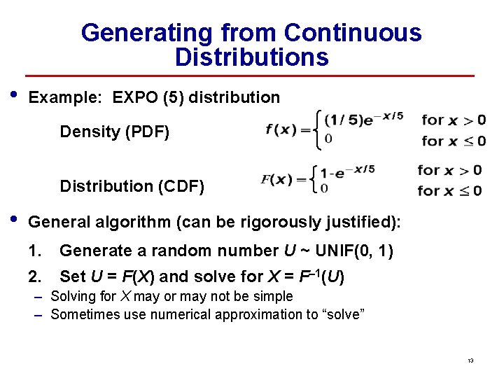
Generating from Continuous Distributions • Example: EXPO (5) distribution Density (PDF) Distribution (CDF) • General algorithm (can be rigorously justified): 1. Generate a random number U ~ UNIF(0, 1) 2. Set U = F(X) and solve for X = F– 1(U) – Solving for X may or may not be simple – Sometimes use numerical approximation to “solve” 13

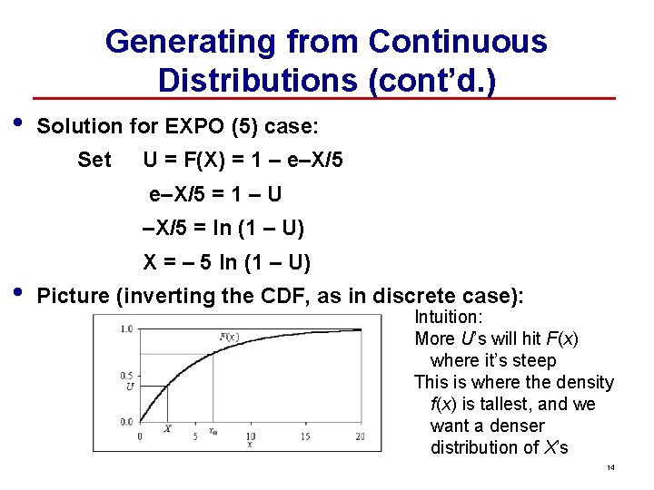
Generating from Continuous Distributions (cont’d. ) • Solution for EXPO (5) case: Set U = F(X) = 1 – e–X/5 = 1 – U –X/5 = ln (1 – U) • X = – 5 ln (1 – U) Picture (inverting the CDF, as in discrete case): Intuition: More U’s will hit F(x) where it’s steep This is where the density f(x) is tallest, and we want a denser distribution of X’s 14

Non-stationary Poisson Processes • • • Many systems have externally originating events affecting them — e. g. , arrivals of customers If process is stationary over time, usually specify a fixed inter-event-time distribution But process could vary markedly in its rate – Fast-food lunch rush – Freeway rush hours Ignoring nonstationarity can lead to serious model and output errors Already seen this — call-center arrivals, Chap. 8 15

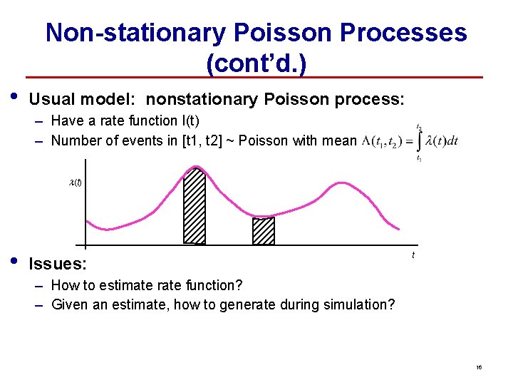
Non-stationary Poisson Processes (cont’d. ) • Usual model: nonstationary Poisson process: – Have a rate function l(t) – Number of events in [t 1, t 2] ~ Poisson with mean l(t) • Issues: t – How to estimate rate function? – Given an estimate, how to generate during simulation? 16

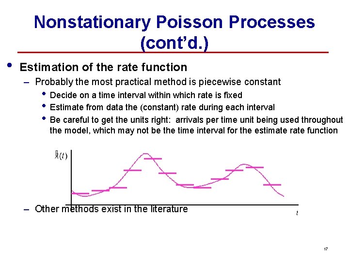
Nonstationary Poisson Processes (cont’d. ) • Estimation of the rate function – Probably the most practical method is piecewise constant • • • Decide on a time interval within which rate is fixed Estimate from data the (constant) rate during each interval Be careful to get the units right: arrivals per time unit being used throughout the model, which may not be the time interval for the estimate rate function – Other methods exist in the literature t 17

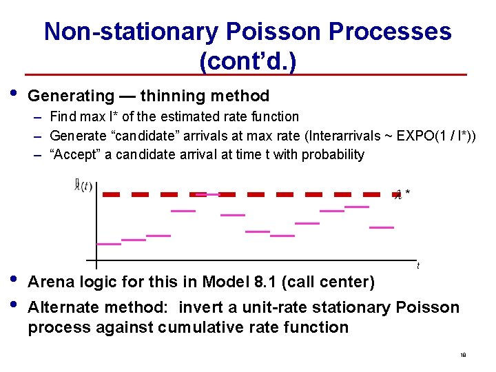
Non-stationary Poisson Processes (cont’d. ) • Generating — thinning method – Find max l* of the estimated rate function – Generate “candidate” arrivals at max rate (Interarrivals ~ EXPO(1 / l*)) – “Accept” a candidate arrival at time t with probability • • t Arena logic for this in Model 8. 1 (call center) Alternate method: invert a unit-rate stationary Poisson process against cumulative rate function 18

Rejection Sampling • For the non-homogeneous Poisson process – we sampled from a process with the maximum rate – then we rejected enough to thin the process down to the correct rate • • This is an example of rejection sampling • Basic Idea Rejection sampling can also be used for sampling from univariate distributions where F-1(x) does not exist or cannot be easily approximate – Sample from another distribution that is easy to sample from – Reject those that are drawn from area where the target distribution has low density Simulation with Arena — Further Statistical Issues 19

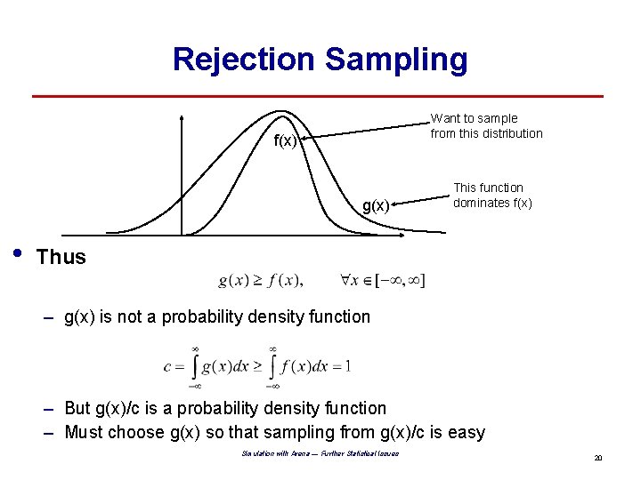
Rejection Sampling Want to sample from this distribution f(x) g(x) • This function dominates f(x) Thus – g(x) is not a probability density function – But g(x)/c is a probability density function – Must choose g(x) so that sampling from g(x)/c is easy Simulation with Arena — Further Statistical Issues 20

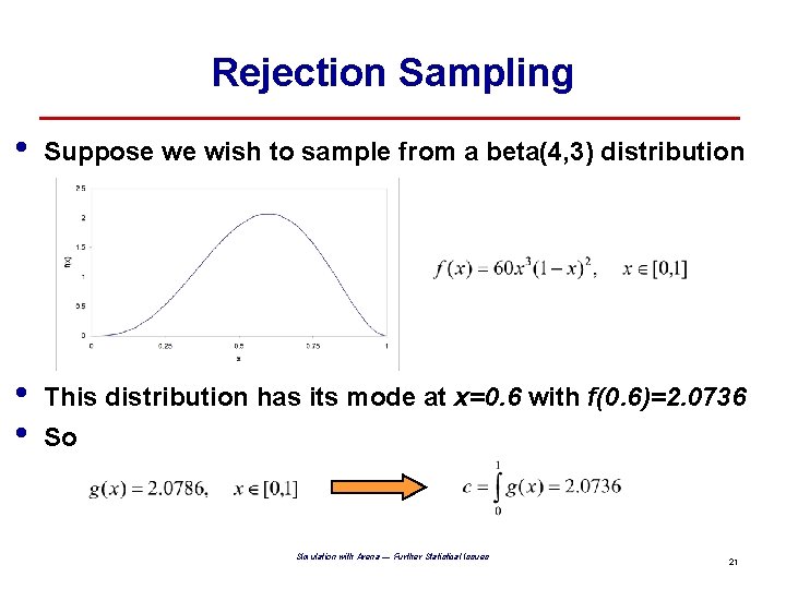
Rejection Sampling • Suppose we wish to sample from a beta(4, 3) distribution • • This distribution has its mode at x=0. 6 with f(0. 6)=2. 0736 So Simulation with Arena — Further Statistical Issues 21

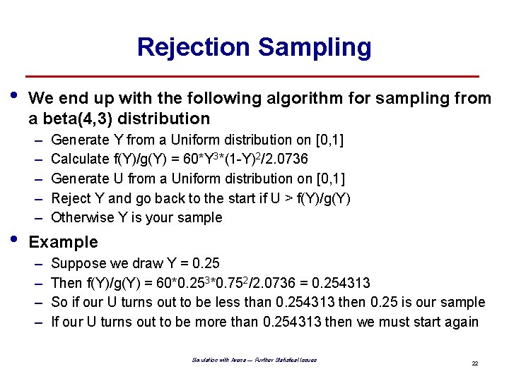
Rejection Sampling • • We end up with the following algorithm for sampling from a beta(4, 3) distribution – – – Generate Y from a Uniform distribution on [0, 1] Calculate f(Y)/g(Y) = 60*Y 3*(1 -Y)2/2. 0736 Generate U from a Uniform distribution on [0, 1] Reject Y and go back to the start if U > f(Y)/g(Y) Otherwise Y is your sample Example – – Suppose we draw Y = 0. 25 Then f(Y)/g(Y) = 60*0. 253*0. 752/2. 0736 = 0. 254313 So if our U turns out to be less than 0. 254313 then 0. 25 is our sample If our U turns out to be more than 0. 254313 then we must start again Simulation with Arena — Further Statistical Issues 22

Variance Reduction • • Random input random output (RIRO) In other words, output has variance – Higher output variance means less precise results – Would like to eliminate or reduce output variance • • One (bad) way to eliminate: replace all input random variables by constants (like their mean) Will get rid of random output, but will also invalidate model Thus, best hope is to reduce output variance Easy (brute-force) variance reduction: just simulate some more – Terminating: additional replications – Steady-state: additional replications or a single, longer run 23

Variance Reduction (cont’d. ) • • • But sometimes can reduce variance without more runs — free lunch (? ) Key: unlike physical experiments, can control randomness in computer-simulation experiments via manipulating the RNG – Re-use the same “random” numbers either as they were, in some opposite sense, or for a similar but simpler model Several different variance-reduction techniques – Classified into categories — common random numbers, antithetic variates, … – Usually requires thorough understanding of model, “code” – Will look only at common random numbers in detail 24

Common Random Numbers (CRN) • • Applies when objective is to compare two (or more) alternative configurations or models – Interest is in difference(s) of performance measure(s) across alternatives – In the PWS, we wanted to test many different configurations of the oil transportation system Intuition: get sharper comparison if you subject all alternatives to the same “conditions” – Then observed differences are due to model differences rather than random differences in the “conditions” – For this PWS this means try out each system configuration with the same simulated traffic arrivals and the same simulated weather patterns 25

Synchronization of Random Numbers in CRN (cont’d. ) • Synchronize by source of randomness (we’ll do) – Assign a stream to each point of variate generation — separate random -number “faucets” • Interarrivals, Part types, Processing times, etc. – Fairly simple but might not ensure complete synchronization • • Something might cause parts to arrive to a Server in a different order across alternatives – Still usually get some benefit from this In PWS Simulation – One file of traffic arrivals – One file of weather variables – Each alternative system design was tested on the same traffic and weather patterns 26

CRN Synchronization by Source (cont’d. ) • • SEEDS module (Elements panel) – Give names to the streams – Common Initialize Option: space seeds within a stream 100, 000 apart between replications to avoid (? ) overlap Use stream assignments (by name) in Arrive, Expressions, and Sequences modules – Append stream name after parameter-value arguments • Expo(12, STREAM 1) 27

CRN Synchronization by Source (cont’d. ) • • We will compare a run using common random numbers to a run with independent random numbers Using SEEDS to force independence across alternatives – Earlier comparison: used default stream (10) for both alternatives A and B but in haphazard unsynchronized way – So results were not independent, but probably not “like vs. like” correlated either, as we’d like for synchronized CRN – To get independence, modify SEEDS module for alternative B to skip streams 1– 15 before naming streams: Model 11. 2 • Can remove place holder for Stream 10: already skipped Simulation with Arena — Further Statistical Issues 28

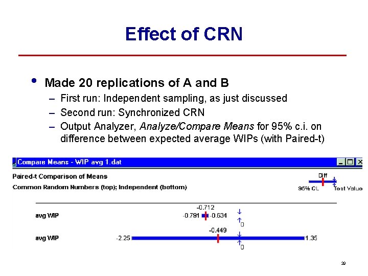
Effect of CRN • Made 20 replications of A and B – First run: Independent sampling, as just discussed – Second run: Synchronized CRN – Output Analyzer, Analyze/Compare Means for 95% c. i. on difference between expected average WIPs (with Paired-t) 29

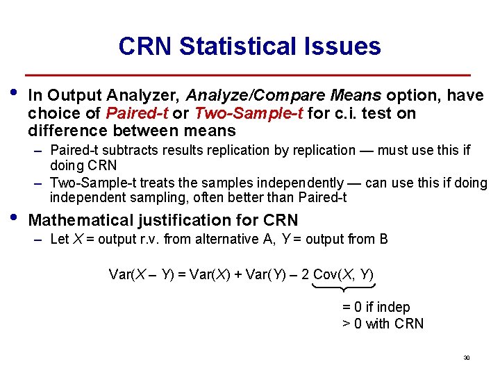
CRN Statistical Issues • • In Output Analyzer, Analyze/Compare Means option, have choice of Paired-t or Two-Sample-t for c. i. test on difference between means – Paired-t subtracts results replication by replication — must use this if doing CRN – Two-Sample-t treats the samples independently — can use this if doing independent sampling, often better than Paired-t Mathematical justification for CRN – Let X = output r. v. from alternative A, Y = output from B Var(X – Y) = Var(X) + Var(Y) – 2 Cov(X, Y) = 0 if indep > 0 with CRN 30

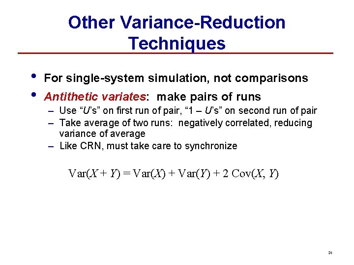
Other Variance-Reduction Techniques • • For single-system simulation, not comparisons Antithetic variates: make pairs of runs – Use “U’s” on first run of pair, “ 1 – U’s” on second run of pair – Take average of two runs: negatively correlated, reducing variance of average – Like CRN, must take care to synchronize Var(X + Y) = Var(X) + Var(Y) + 2 Cov(X, Y) 31