Generalized Hough Transform The Generalized Hough Transform From


")


 over the range (0, 2π) in")
 and rotation ( )")


- Slides: 65
Generalized Hough Transform
The Generalized Hough Transform
From Standard to Generalized HT 1. Standard Hough Transform requires parametric representation for desired curve 2. This idea is generalized in the Generalized Hough Transform
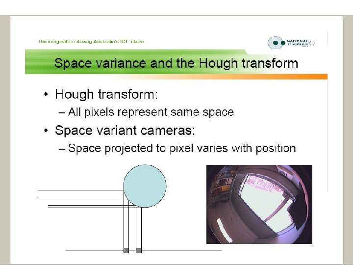
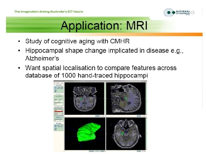
Example: Human Face recognition • Is there some attribute of the structure of the head that we can exploit to help estimate pose estimation? • Is this attribute invariant under change in pose? – Or • “Can we model how this attribute varies with pose? ”
Hough Transform in General 1. Technique to isolate curves of a given shape in an image 2. Standard Hough Transform (HT) uses parametric formulation of curves 3. Generalized Hough Transform (GHT) extends for arbitrary curves
1. Key Idea to improve correlation by voting When we compute the correlation by voting, we spend most of the time casting bad votes. 2. Idea is to use extra shape information (e. g. gradients) gradients to cast fewer votes: 1. O(n) complexity: For each of O(n) points on the boundary, cast O(1) votes.
General Hough Algorithm Idea • 1. explicitly list points on shape • 2. make table for all edge pixels for target • 3. for each pixel store its position relative to some reference point on the shape – ‘if I’m pixel i on the boundary, the reference point is at ref[i]’
The Generalized Hough Transform 1. Technique to find arbitrary curves in a given image 2. Parametric equation no longer required 3. Look-up table used as transform mechanism 4. Two phases: 1. R-Table Generation phase 2. Object Detection phase
The Generalized Hough Transform 1. Standard Techniques allow for invariance to scale and rotation in the plane 2. In general, objects in the real world are 3 dimensional 3. Hence a single silhouette provides no invariance to pose (i. e. rotation out of the plane). 4. No pose estimation. 5. This is generalized to Surface Normal Hough Transform
Building the R-Table in GHT
GHT: Building the R-Table 1. We are given the shape we want to localize 2. We build a lookup table for this shape, called R-Table It will replace the need for a parametric equation in the transform stage
GHT: Building the R-Table
GHT: Building the R-Table
GHT: Building R-Table GHT: Building the R-Table
Object Localization in the R-Table in GHT
GHT: Object Localization
GHT: Object Localization
GHT: Object Localization
Conclusions on GHT 1. Standard Techniques allow for invariance to scale and rotation in the plane 2. In general, objects in the real world are 3 -dimensional 3. Hence a single silhuette provides no invariance to pose (i. e. rotation out of the plane). 4. No pose estimation. 5. Now show more details
Generalized Hough Transform Algorithm
Algorithm of the General Hough Transform
Hough Transform for Curves • The H. T. can be generalized to detect any curve that can be expressed in parametric form: – Y = f(x, a 1, a 2, …ap) – a 1, a 2, … ap are the parameters – The parameter space is p-dimensional – The accumulating array is LARGE!
Generalized Hough Transform algorithm • Find all desired points in image • For each feature point – for each pixel i on target boundary • get relative position of reference point from i • add this offset to position of i • increment that position in accumulator • Find local maxima in accumulator • Map maxima back to image to view
Generalizing the H. T. The H. T. can be used even if the curve has not a simple analytic form! (xc, yc) fi ai Pi xc = xi + ricos(ai) ri yc = yi + risin(ai) 1. Pick a reference point (xc, yc) 2. For i = 1, …, n : 1. Draw segment to Pi on the boundary. 2. Measure its length ri, and its orientation ai. 3. Write the coordinates of (xc, yc) as a function of ri and ai 4. Record the gradient orientation fi at Pi. 3. Build a table with the data, indexed by fi.
Generalizing the H. T. Suppose, there were m different gradient orientations: (m <= n) aj rj fj (xc, yc) ri fi ai Pi xc = xi + ricos(ai) yc = yi + risin(ai) f 1 (r 11, a 11), (r 12, a 12), …, (r 1 n 1, a 1 n 1) f 2 (r 21, a 21), (r 22, a 12), …, (r 2 n 2, a 1 n 2) . . . fm (rm 1, am 1), (rm 2, am 2), …, (rmnm, amnm) H. T. table
Generalized H. T. Algorithm: Finds a rotated, scaled, and translated version of the curve: 1. reference points (xc, yc), scaling factor S arjj f j q S Pj fi r iai ) S , y c Pi c x ( Form an A accumulator array of possible and Rotation angle q. 2. q For each edge (x, y) in the image: 1. 2. For each (r, a) corresponding to f(x, y) do: fi q k a r k S Pk 1. xc = xi + ricos(ai) yc = yi + risin(ai) Compute f(x, y) 3. For each S and q: 1. 2. xc = xi + r(f) S cos[a(f) + q] 3. A(xc, yc, S, q) = A(xc, yc, S, q) + 1 yc = yi + r(f) S sin[a(f) + q] Find maxima of A.
Another variant of the Generalized Hough Transform Find Object Center given edges Create Accumulator Array Initialize: For each edge point For each entry in table, compute: Increment Accumulator: Find Local Maxima in
Generalize HT applied for circuits
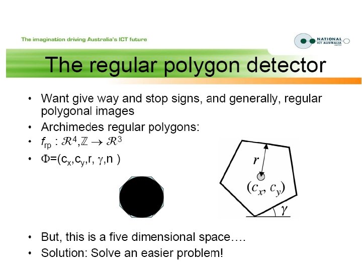
Properties of Generalized Hough Transform • What can we do when the curve we want to detect is not easily described parametrically? 1. ~ By this, we mean, it cannot be captured in a relatively small number of parameters. 2. ~ Recall, the dimensionality of the Hough space equal the number of parameters! • The GHT constructs a parametric description of an arbitrary shape based on a learning process. • This parametric description is not, in general, compact. • We will begin by assuming the size, shape, and rotation (orientation) of the region is known a priori. (Or that we want only to detect instances of a given size and orientation. 1. ~ The voting space is (equivalent to) image space, 2 D, and rotation. 2. ~ We will see how to deal with unknown orientation and size shortly -- with a 4 D Hough space. in the case of known size
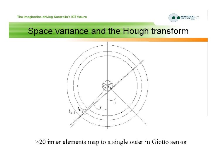
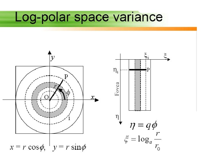
: An arbitrary reference point inside the shape. : The length of the j-th line from the reference point to the shape perimeter, intersecting at a point of tangent angle ø. : The angle of the (current) tangent(s) to the perimeter. : The orientation of the j-th line segment. The list of ( , ) pairs, for a given and a partial characterization of the shape. constitutes
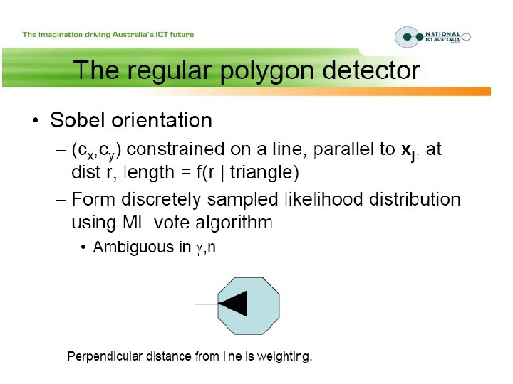
• By sweeping the tangent angle (ø) over the range (0, 2π) in some reasonable quantization (!), we build what is called the R-table (reference table) description of the shape. • Each pixel x (say, a detected edge point) with local orientation ø provides evidence (votes for) reference points at the set of locations indicated by the list in the R-table for that tangent direction. . . • A vote is cast for each (r , ) pair in the list for that ø value. The voting space is isomorphic to image space. • Again, this assumes known size and orientation for all appearances of the shape. • After all the edge points have voted for all of their possible reference points, we interrogate the voting space for significant local maxima. These suggest possible detections of the shape of interest.
• If we have not prenormalized for size (S) and rotation ( ) then our voting space is four dimensional and the reference location receiving the vote(s) for a given edge point and R-table entry is: • Now, we interrogate the 4 D accumulator array to recover likely locations, scale, and orientation for appearances of the shape. • This is really a fancy form of a template match -- but one that is far more robust than a straightforward template matching algorithm. • Selecting among multiple possible shapes requires multiple R-tables, multiple voting spaces. • But, so does looking for lines and circles in the same image. .
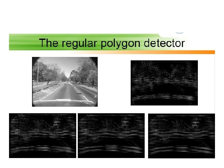
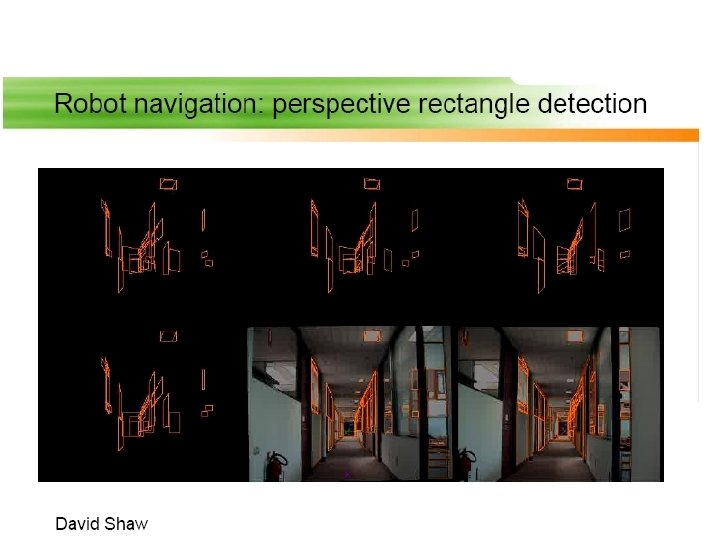
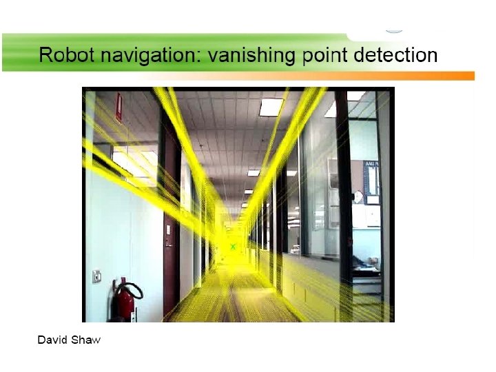
Generalized HT in biologically motivated robotics
Bimodal Active Stereo
Many simultaneous problems in robotics
Research Philosophy
The main concept of Radon Transform
The main concept of Radon Transform
Hough Transform: Comments • Works on Disconnected Edges • Relatively insensitive to occlusion • Effective for simple shapes (lines, circles, etc) • Trade-off between work in Image Space and Parameter Space • Handling inaccurate edge locations: • Increment Patch in Accumulator rather than a single point
H. T. Summary • H. T. is a “voting” scheme – points vote for a set of parameters describing a line or curve. • The more votes for a particular set – the more evidence that the corresponding curve is present in the image. • Can detect MULTIPLE curves in one shot. • Computational cost increases with the number of parameters describing the curve. end