Generalized Hidden Markov Models for Eukaryotic gene prediction

Generalized Hidden Markov Models for Eukaryotic gene prediction CBB 231 / COMPSCI 261 W. H. Majoros

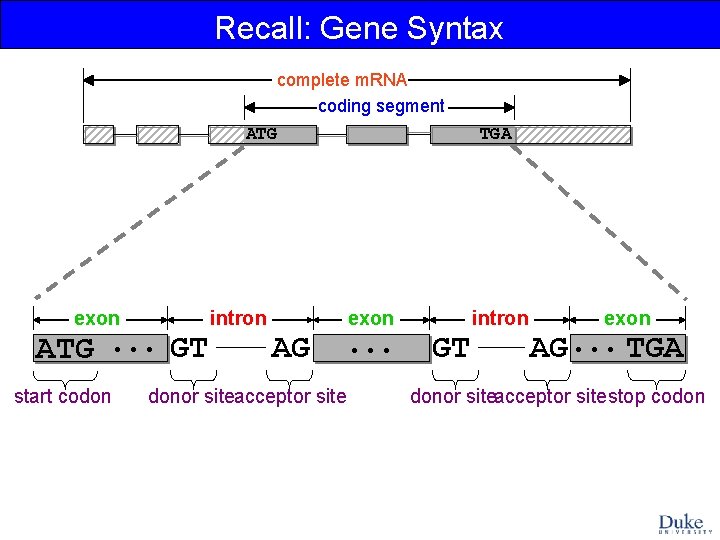
Recall: Gene Syntax complete m. RNA coding segment ATG exon ATG. . . GT start codon intron TGA exon AG donor siteacceptor site . . . intron GT exon AG. . . TGA donor siteacceptor sitestop codon

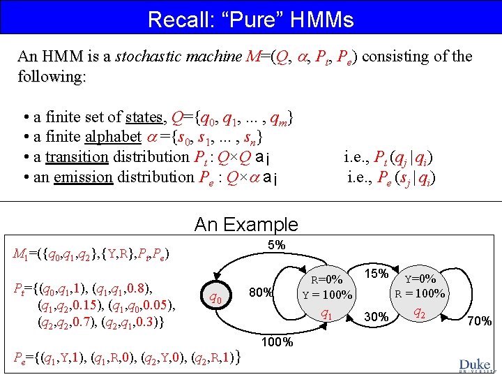
Recall: “Pure” HMMs An HMM is a stochastic machine M=(Q, , Pt, Pe) consisting of the An HMM is a following: • a finite set of states, Q={q 0, q 1, . . . , qm} • a finite alphabet ={s 0, s 1, . . . , sn} • a transition distribution Pt : Q×Q a¡ • an emission distribution Pe : Q× a¡ i. e. , Pt (qj | qi) i. e. , Pe (sj | qi) An Example 5% M 1=({q 0, q 1, q 2}, {Y, R}, Pt, Pe) Pt={(q 0, q 1, 1), (q 1, 0. 8), (q 1, q 2, 0. 15), (q 1, q 0, 0. 05), (q 2, 0. 7), (q 2, q 1, 0. 3)} q 0 Pe={(q 1, Y, 1), (q 1, R, 0), (q 2, Y, 0), (q 2, R, 1)} 80% 15% Y=0% R = 100% Y = 100% q 1 100% 30% q 2 70%

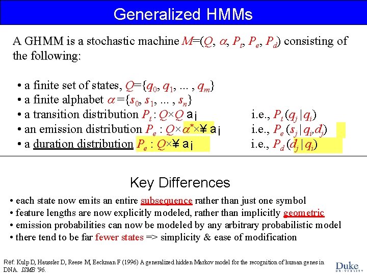
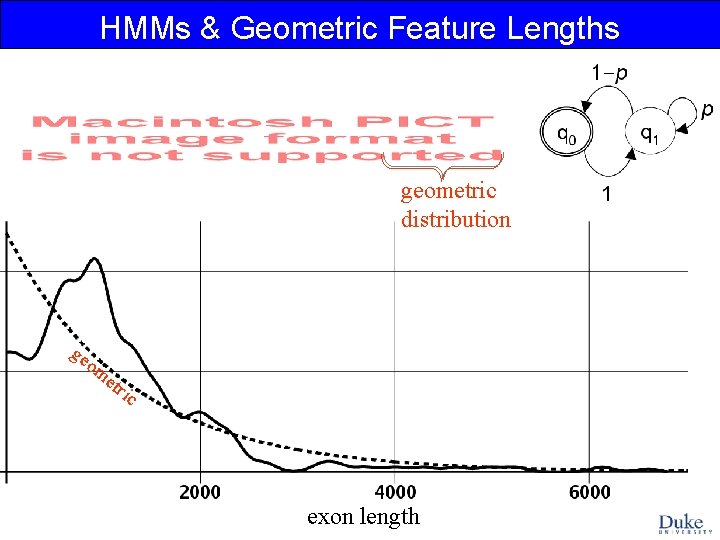
Generalized HMMs A GHMM is a stochastic machine M=(Q, , Pt, Pe, Pd) consisting of A GHMM is a the following: • a finite set of states, Q={q 0, q 1, . . . , qm} • a finite alphabet ={s 0, s 1, . . . , sn} • a transition distribution Pt : Q×Q a¡ • an emission distribution Pe : Q× *×¥ a¡ • a duration distribution Pe : Q×¥ a¡ i. e. , Pt (qj | qi) i. e. , Pe (sj | qi, dj) i. e. , Pd (dj | qi) Key Differences • each state now emits an entire subsequence rather than just one symbol • feature lengths are now explicitly modeled, rather than implicitly geometric • emission probabilities can now be modeled by any arbitrary probabilistic model • there tend to be far fewer states => simplicity & ease of modification Ref: Kulp D, Haussler D, Reese M, Eeckman F (1996) A generalized hidden Markov model for the recognition of human genes in DNA. ISMB '96.

HMMs & Geometric Feature Lengths geometric distribution ge om e tri c exon length

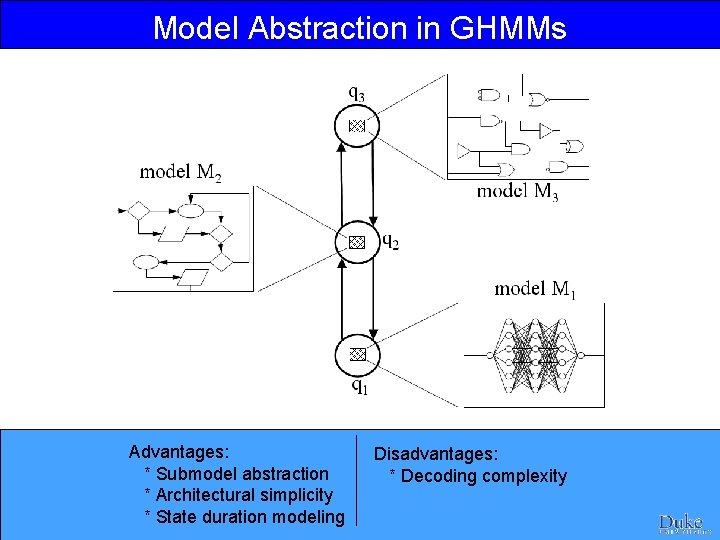
Model Abstraction in GHMMs Advantages: * Submodel abstraction * Architectural simplicity * State duration modeling Disadvantages: * Decoding complexity

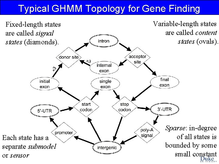
Typical GHMM Topology for Gene Finding Fixed-length states are called signal states (diamonds). Each state has a separate submodel or sensor Variable-length states are called content states (ovals). Sparse: in-degree of all states is bounded by some small constant

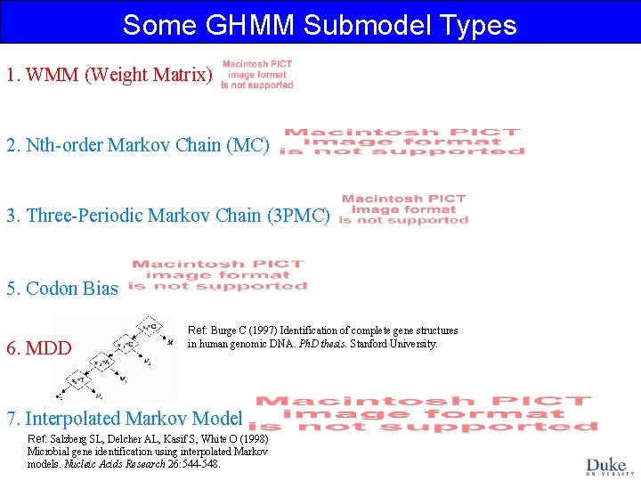
Some GHMM Submodel Types 1. WMM (Weight Matrix) 2. Nth-order Markov Chain (MC) 3. Three-Periodic Markov Chain (3 PMC) 5. Codon Bias 6. MDD Ref: Burge C (1997) Identification of complete gene structures in human genomic DNA. Ph. D thesis. Stanford University. 7. Interpolated Markov Model Ref: Salzberg SL, Delcher AL, Kasif S, White O (1998) Microbial gene identification using interpolated Markov models. Nucleic Acids Research 26: 544 -548.

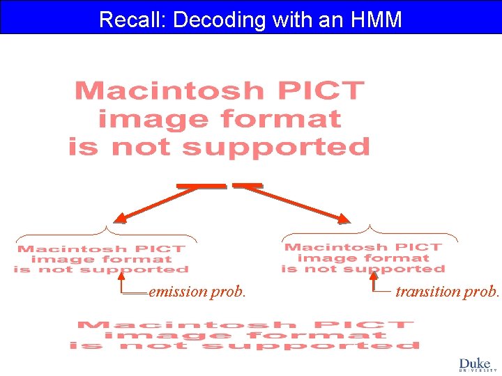
Recall: Decoding with an HMM emission prob. transition prob.

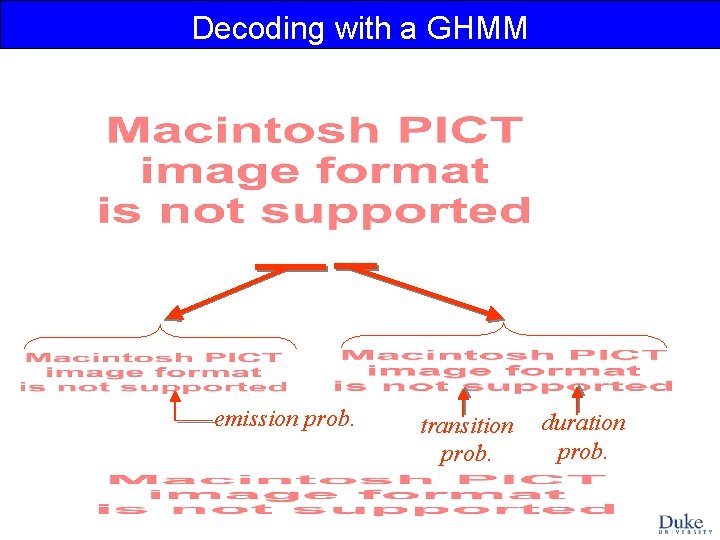
Decoding with a GHMM emission prob. transition prob. duration prob.

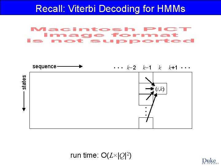
Recall: Viterbi Decoding for HMMs . . . k-2 k-1 states sequence k (i, k) . . . run time: O(L×|Q|2) k+1 . . .

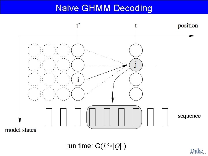
Naive GHMM Decoding run time: O(L 3×|Q|2)

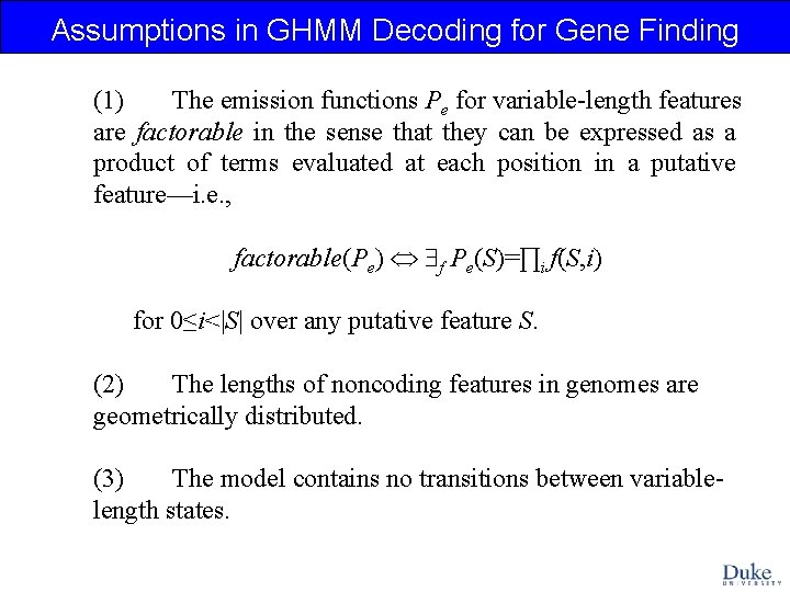
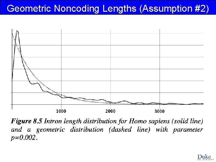
Assumptions in GHMM Decoding for Gene Finding (1) The emission functions Pe for variable-length features are factorable in the sense that they can be expressed as a product of terms evaluated at each position in a putative feature—i. e. , factorable(Pe) f Pe(S)=∏i f(S, i) for 0≤i<|S| over any putative feature S. (2) The lengths of noncoding features in genomes are geometrically distributed. (3) The model contains no transitions between variablelength states.

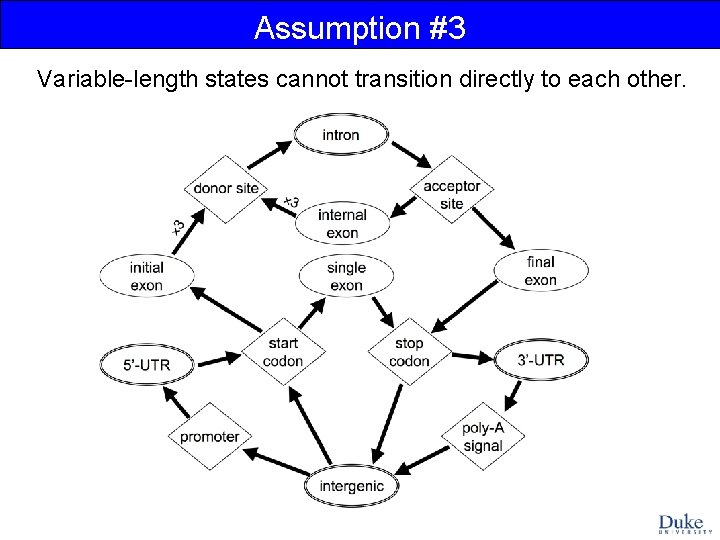
Assumption #3 Variable-length states cannot transition directly to each other.

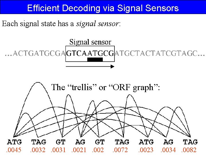
Efficient Decoding via Signal Sensors Each signal state has a signal sensor: The “trellis” or “ORF graph”: . 0045 . 0032 . 0031 . 002 . 0072 . 0023 . 0034 . 0082

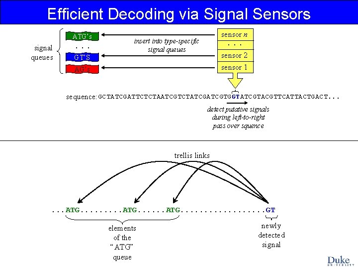
Efficient Decoding via Signal Sensors ATG’s signal queues . . . sensor n . . . insert into type-specific signal queues sensor 2 sensor 1 GT’S AG’s sequence: GCTATCGATTCTCTAATCGTCTATCGTGGTATCGTACGTTCATTACTGACT. . . detect putative signals during left-to-right pass over squence trellis links . . . ATG. . . . . GT elements of the “ATG” queue newly detected signal

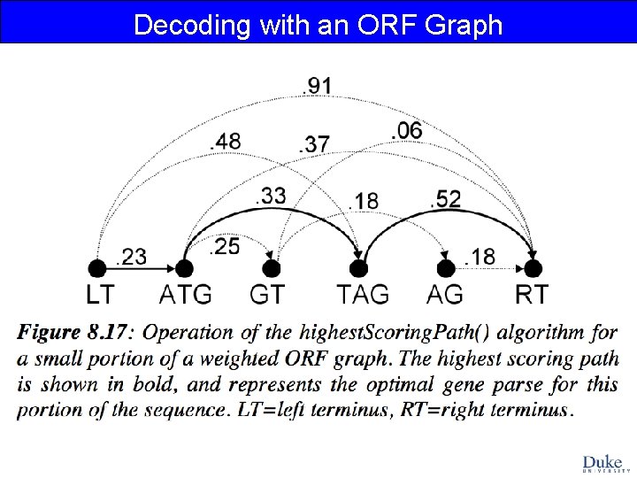
Decoding with an ORF Graph

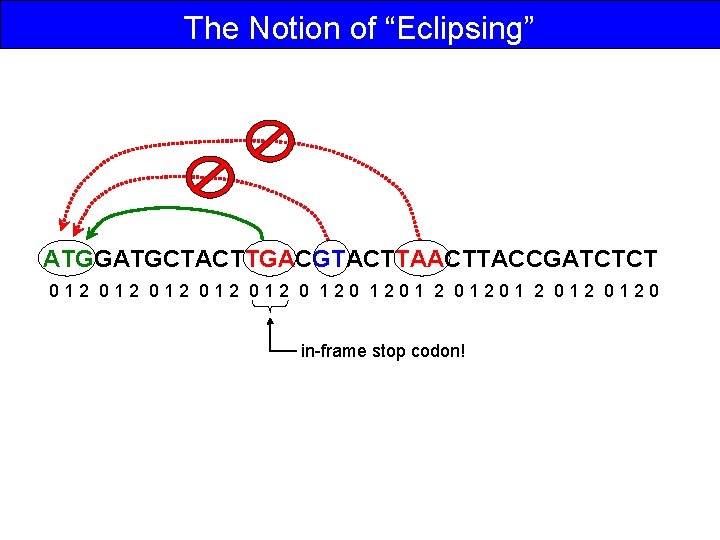
The Notion of “Eclipsing” ATGGATGCTACTTGACGTACTTACCGATCTCT 012 012 012 0 1201 2 012 0120 in-frame stop codon!

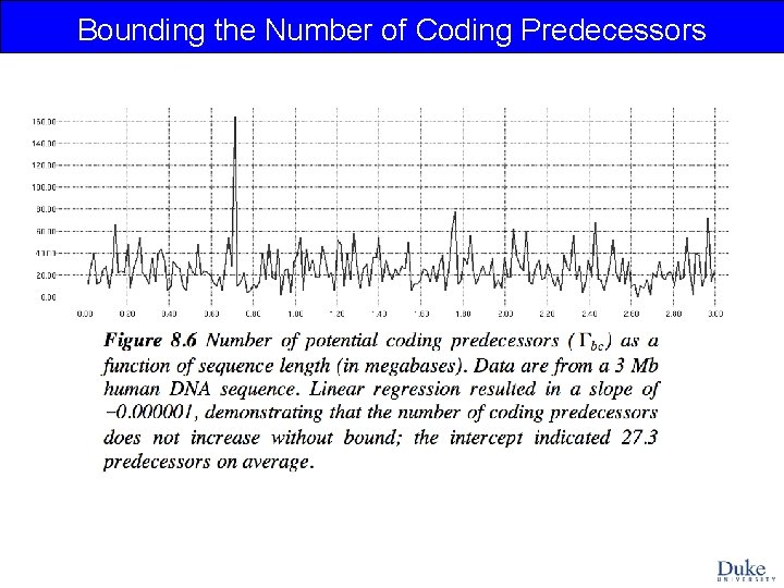
Bounding the Number of Coding Predecessors

Geometric Noncoding Lengths (Assumption #2)

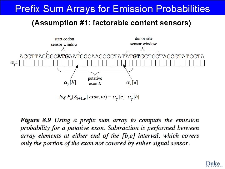
Prefix Sum Arrays for Emission Probabilities (Assumption #1: factorable content sensors)

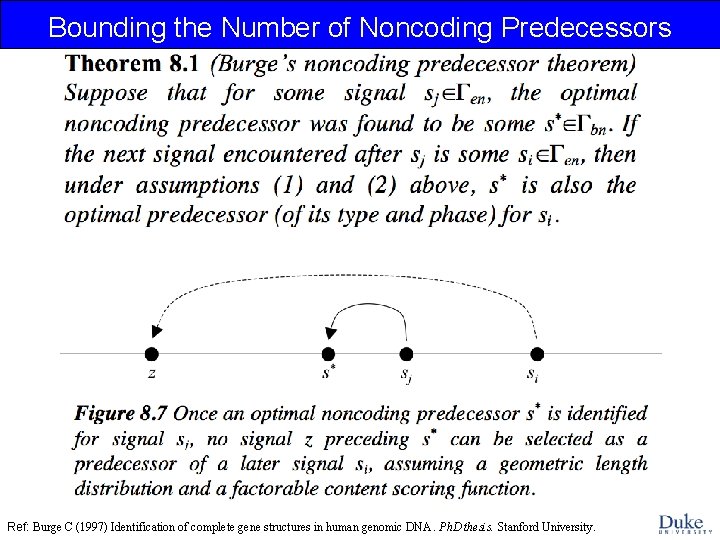
Bounding the Number of Noncoding Predecessors Ref: Burge C (1997) Identification of complete gene structures in human genomic DNA. Ph. D thesis. Stanford University.

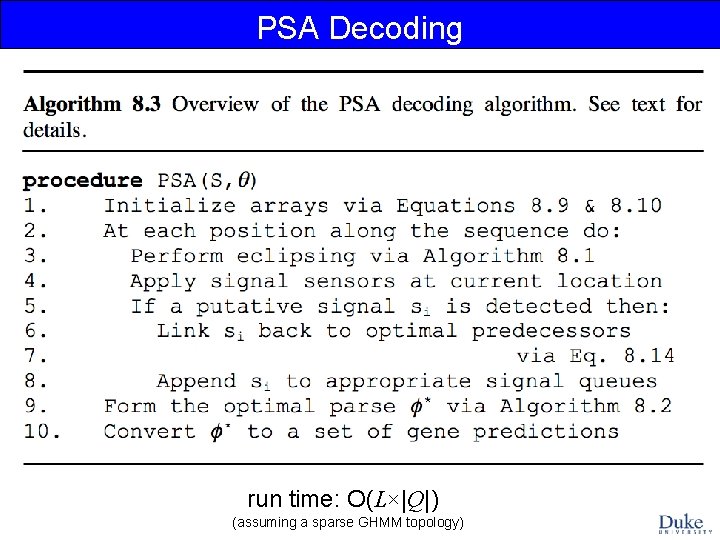
PSA Decoding run time: O(L×|Q|) (assuming a sparse GHMM topology)

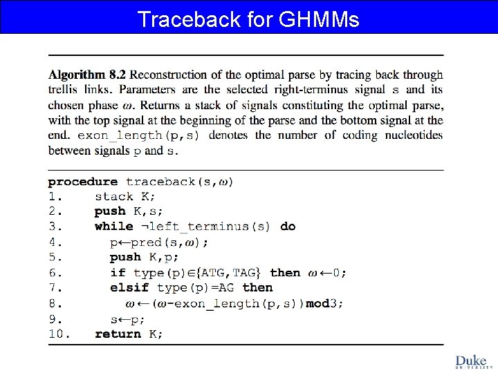
Traceback for GHMMs

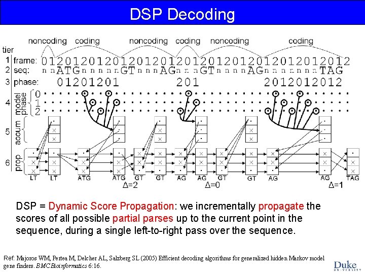
DSP Decoding DSP = Dynamic Score Propagation: we incrementally propagate the scores of all possible partial parses up to the current point in the sequence, during a single left-to-right pass over the sequence. Ref: Majoros WM, Pertea M, Delcher AL, Salzberg SL (2005) Efficient decoding algorithms for generalized hidden Markov model gene finders. BMC Bioinformatics 6: 16.

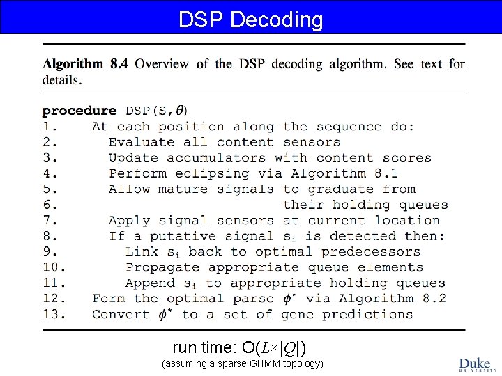
DSP Decoding run time: O(L×|Q|) (assuming a sparse GHMM topology)

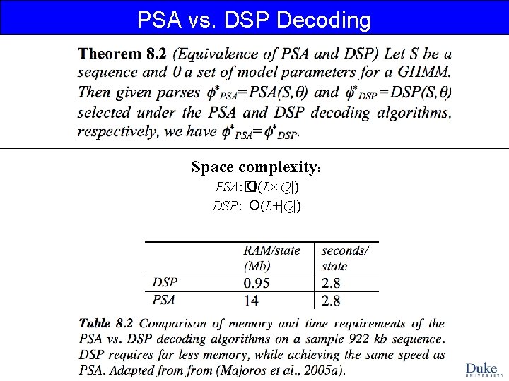
PSA vs. DSP Decoding Space complexity: PSA: � O(L×|Q|) DSP: O(L+|Q|)

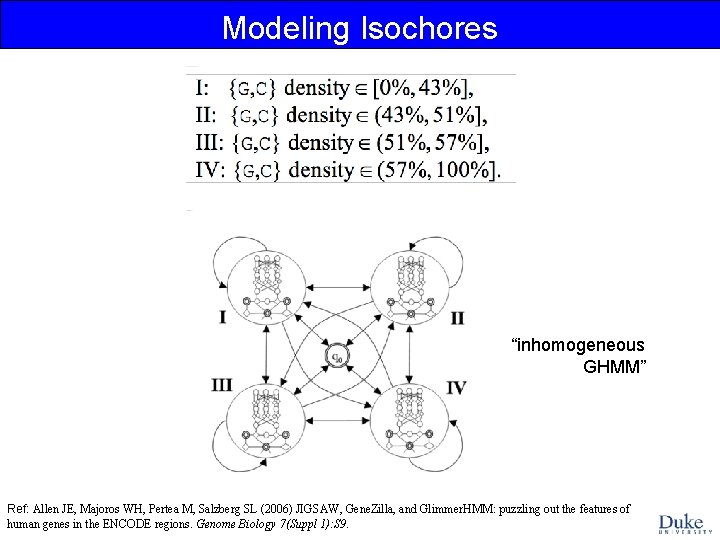
Modeling Isochores “inhomogeneous GHMM” Ref: Allen JE, Majoros WH, Pertea M, Salzberg SL (2006) JIGSAW, Gene. Zilla, and Glimmer. HMM: puzzling out the features of human genes in the ENCODE regions. Genome Biology 7(Suppl 1): S 9.

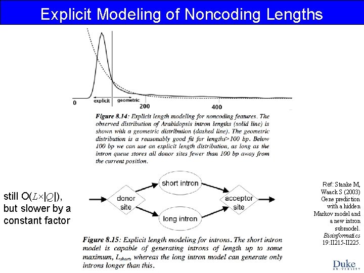
Explicit Modeling of Noncoding Lengths still O(L×|Q|), but slower by a constant factor Ref: Stanke M, Waack S (2003) Gene prediction with a hidden Markov model and a new intron submodel. Bioinformatics 19: II 215 -II 225.

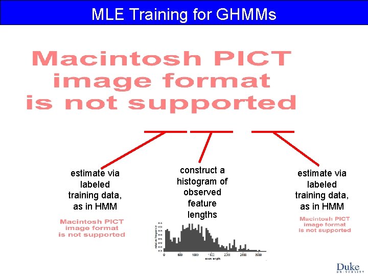
MLE Training for GHMMs estimate via labeled training data, as in HMM construct a histogram of observed feature lengths estimate via labeled training data, as in HMM

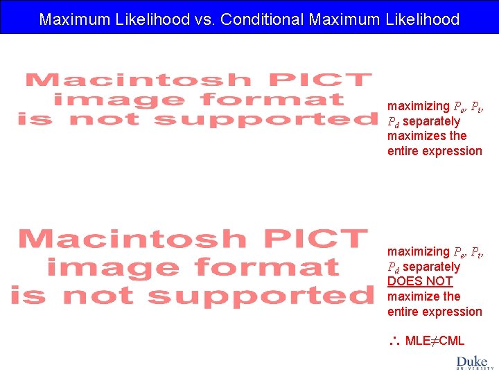
Maximum Likelihood vs. Conditional Maximum Likelihood maximizing Pe, Pt, Pd separately maximizes the entire expression maximizing Pe, Pt, Pd separately DOES NOT maximize the entire expression MLE≠CML

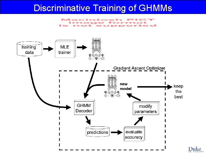
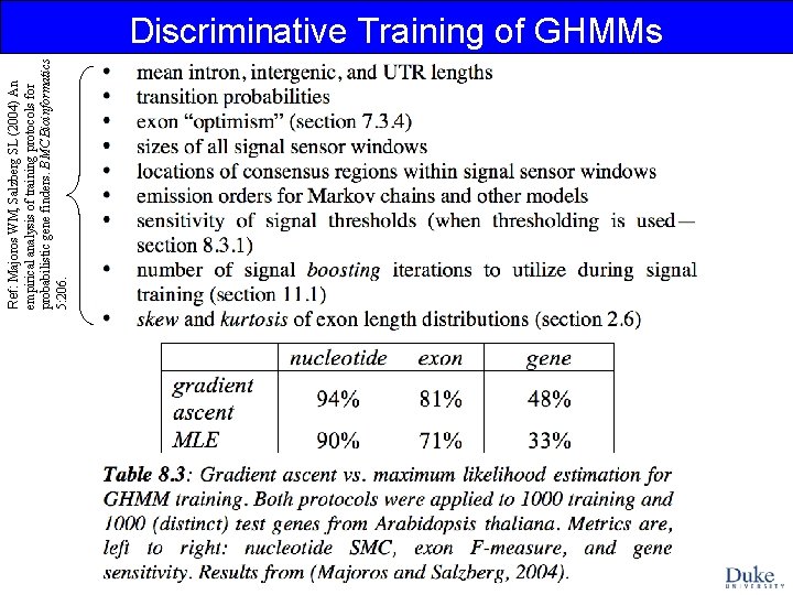
Discriminative Training of GHMMs

Ref: Majoros WM, Salzberg SL (2004) An empirical analysis of training protocols for probabilistic gene finders. BMC Bioinformatics 5: 206. Discriminative Training of GHMMs

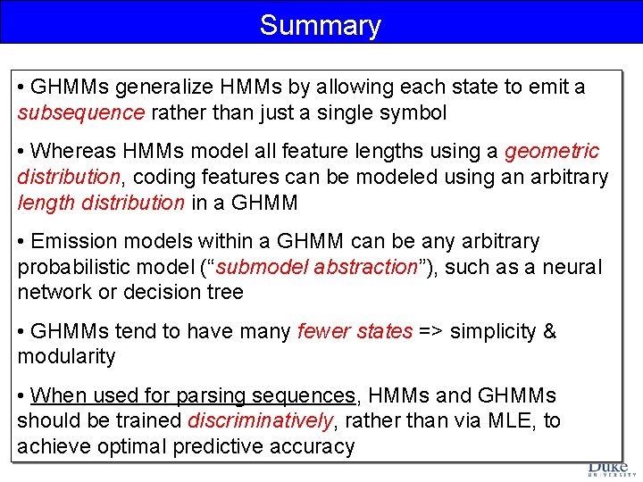
Summary • GHMMs generalize HMMs by allowing each state to emit a subsequence rather than just a single symbol • Whereas HMMs model all feature lengths using a geometric distribution, coding features can be modeled using an arbitrary length distribution in a GHMM • Emission models within a GHMM can be any arbitrary probabilistic model (“submodel abstraction”), such as a neural network or decision tree • GHMMs tend to have many fewer states => simplicity & modularity • When used for parsing sequences, HMMs and GHMMs should be trained discriminatively, rather than via MLE, to achieve optimal predictive accuracy