Generalized Finite Element Methods Approximation LS and MLS

Generalized Finite Element Methods Approximation (LS and MLS) Suvranu De

Last class Interpolation Polynomial interpolation Lagrange form Newton form Interpolation error estimate Piecewise polynomial interpolation (the finite element idea) in 1 and 2 D and the route to FEM Hermite interpolation

This class Approximation vs Interpolation Least squares approximation (LS) Moving Least squares approximation (MLS) and the route to meshfree methods

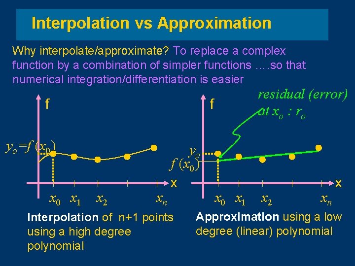
Interpolation vs Approximation Why interpolate/approximate? To replace a complex function by a combination of simpler functions …. so that numerical integration/differentiation is easier f residual (error) at xo : ro f yo=f (x 0) x 0 x 1 x 2 xn yo f (x 0) x Interpolation of n+1 points using a high degree polynomial x 0 x 1 x 2 xn x Approximation using a low degree (linear) polynomial

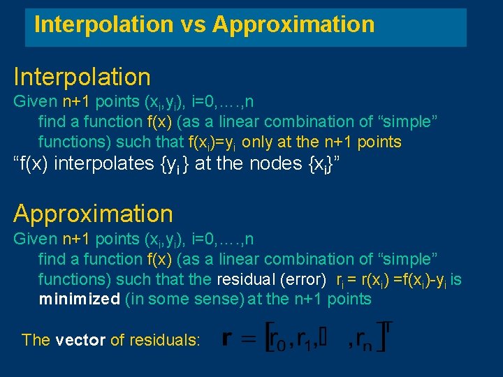
Interpolation vs Approximation Interpolation Given n+1 points (xi, yi), i=0, …. , n find a function f(x) (as a linear combination of “simple” functions) such that f(xi)=yi only at the n+1 points “f(x) interpolates {yi } at the nodes {xi}” Approximation Given n+1 points (xi, yi), i=0, …. , n find a function f(x) (as a linear combination of “simple” functions) such that the residual (error) ri = r(xi) =f(xi)-yi is minimized (in some sense) at the n+1 points The vector of residuals:

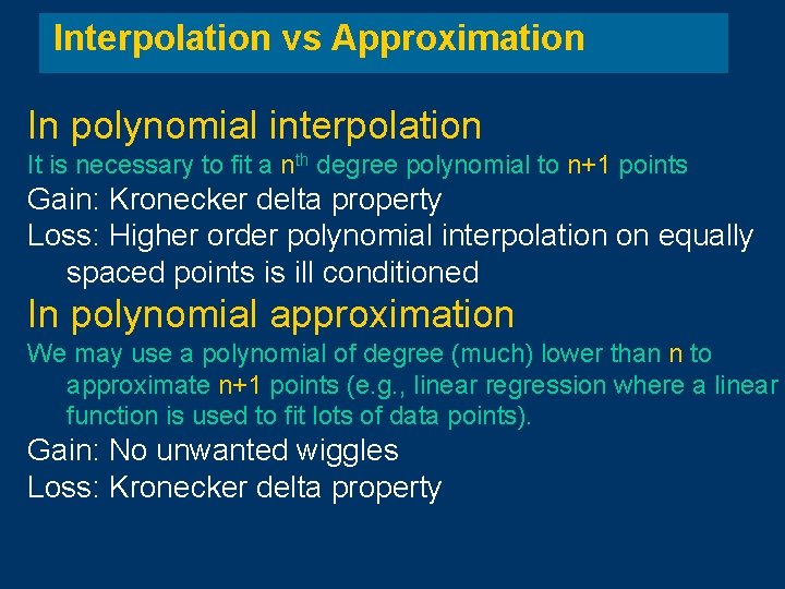
Interpolation vs Approximation In polynomial interpolation It is necessary to fit a nth degree polynomial to n+1 points Gain: Kronecker delta property Loss: Higher order polynomial interpolation on equally spaced points is ill conditioned In polynomial approximation We may use a polynomial of degree (much) lower than n to approximate n+1 points (e. g. , linear regression where a linear function is used to fit lots of data points). Gain: No unwanted wiggles Loss: Kronecker delta property

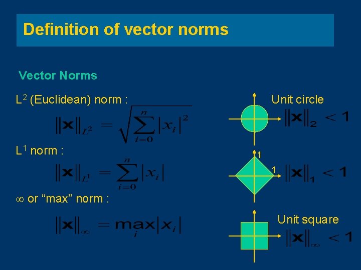
Definition of vector norms Vector Norms L 2 (Euclidean) norm : L 1 norm : Unit circle 1 1 or “max” norm : Unit square

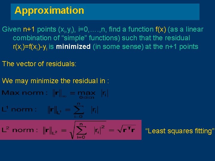
Approximation Given n+1 points (xi, yi), i=0, …. , n, find a function f(x) (as a linear combination of “simple” functions) such that the residual r(xi)=f(xi)-yi is minimized (in some sense) at the n+1 points The vector of residuals: We may minimize the residual in : “Least squares fitting”

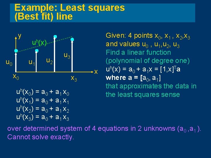
Example: Least squares (Best fit) line y u 0 uh(x) u 1 u 2 u 3 x 0 uh(x 0) = a 0 + a 1 x 0 uh(x 1) = a 0 + a 1 x 1 uh(x 2) = a 0 + a 1 x 2 uh(x 3) = a 0 + a 1 x 3 x Given: 4 points x 0, x 1 , x 2, x 3 and values u 0 , u 1, u 2, u 3 Find a linear function (polynomial of degree one) uh(x) = a 0 + a 1 x = [1, x]Ta where a = [a 0, a 1] that approximates the data in the least squares sense over determined system of 4 equations in 2 unknowns (a 0 , a 1 ). Cannot solve exactly.

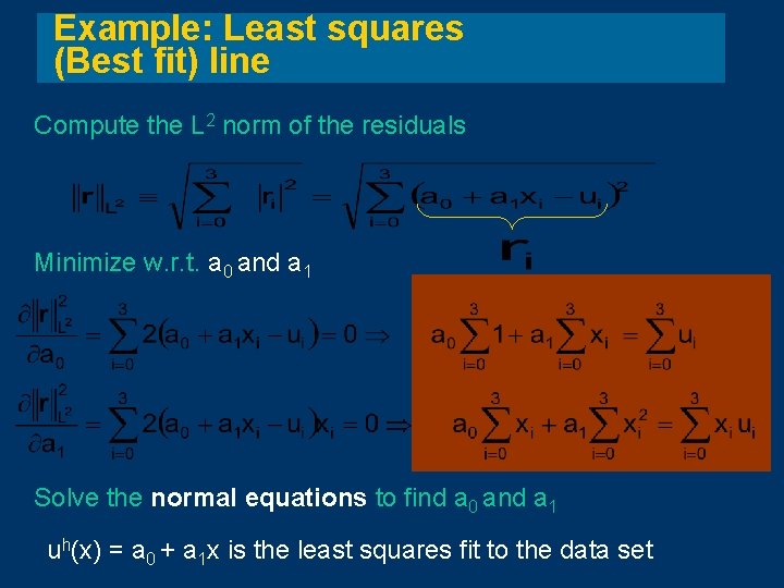
Example: Least squares (Best fit) line Compute the L 2 norm of the residuals Minimize w. r. t. a 0 and a 1 Solve the normal equations to find a 0 and a 1 uh(x) = a 0 + a 1 x is the least squares fit to the data set

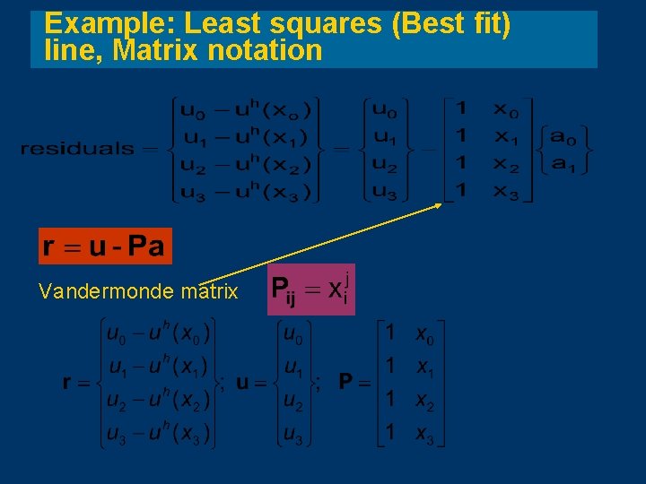
Example: Least squares (Best fit) line, Matrix notation Vandermonde matrix

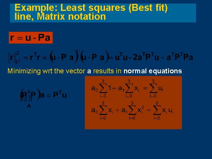
Example: Least squares (Best fit) line, Matrix notation Minimizing wrt the vector a results in normal equations

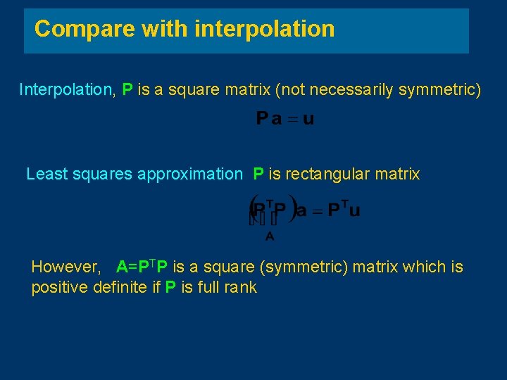
Compare with interpolation Interpolation, P is a square matrix (not necessarily symmetric) Least squares approximation P is rectangular matrix However, A=PTP is a square (symmetric) matrix which is positive definite if P is full rank

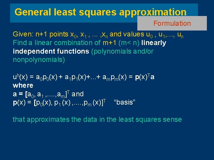
General least squares approximation Formulation Given: n+1 points x 0, x 1 , . . . , xn and values u 0 , u 1, . . . , un Find a linear combination of m+1 (m< n) linearly independent functions (polynomials and/or nonpolynomials) uh(x) = a 0 p 0(x) + a 1 p 1(x)+. . . + ampm(x) = p(x)Ta where a = [a 0, a 1 , . . , am]T and p(x) = [p 0(x), p 1 (x) , . . , pm (x)]T “basis” that approximates the data in the least squares sense

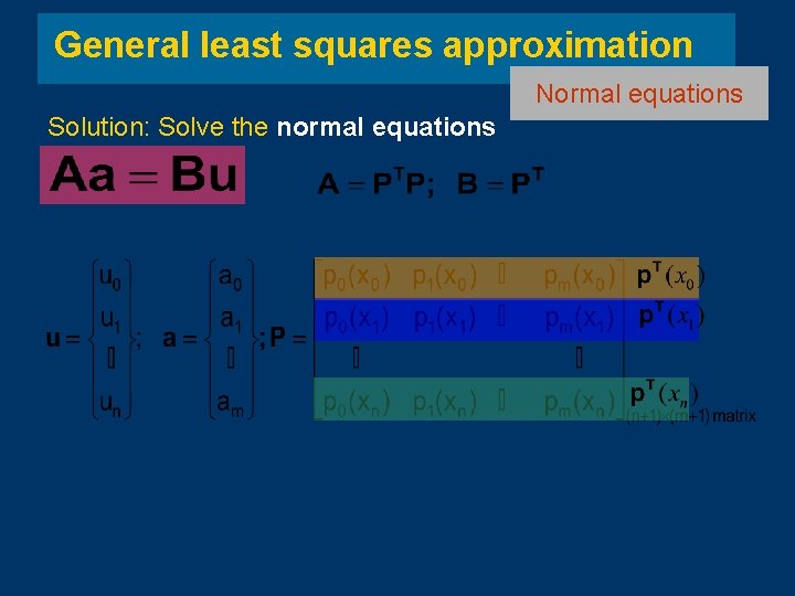
General least squares approximation Normal equations Solution: Solve the normal equations

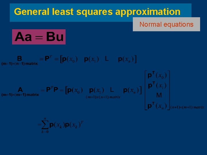
General least squares approximation Normal equations

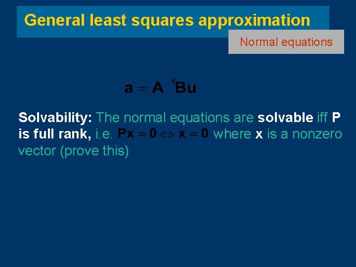
General least squares approximation Normal equations Solvability: The normal equations are solvable iff P is full rank, i. e. where x is a nonzero vector (prove this)

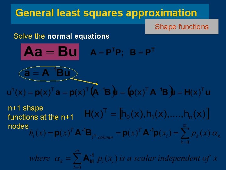
General least squares approximation Shape functions Solve the normal equations n+1 shape functions at the n+1 nodes

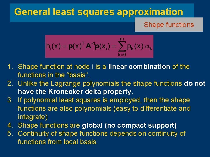
General least squares approximation Shape functions 1. Shape function at node i is a linear combination of the functions in the “basis”. 2. Unlike the Lagrange polynomials the shape functions do not have the Kronecker delta property. 3. If polynomial least squares is employed, then the shape functions are also polynomials (easy to differentiate and integrate) 4. Shape functions are global (no compact support) 5. Continuity of shape functions depends on continuity of functions from local basis.

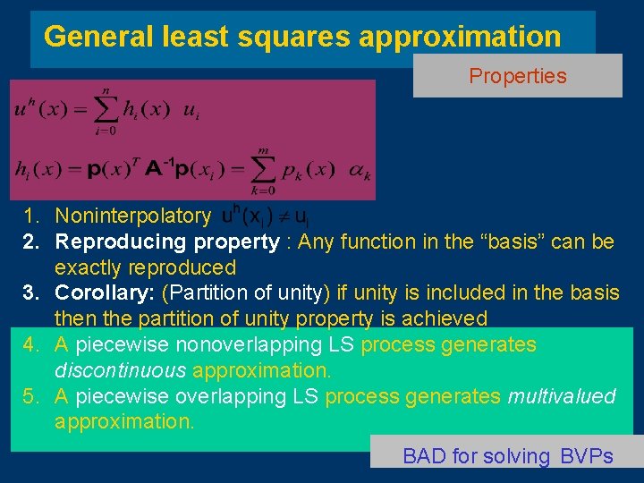
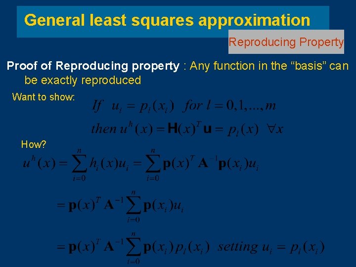
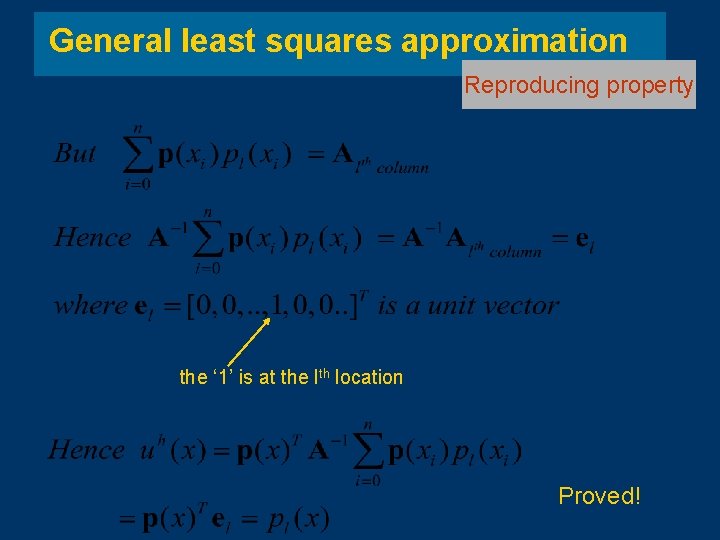
General least squares approximation Properties 1. Noninterpolatory 2. Reproducing property : Any function in the “basis” can be exactly reproduced 3. Corollary: (Partition of unity) if unity is included in the basis then the partition of unity property is achieved 4. A piecewise nonoverlapping LS process generates discontinuous approximation. 5. A piecewise overlapping LS process generates multivalued approximation. BAD for solving BVPs

General least squares approximation Reproducing Property Proof of Reproducing property : Any function in the “basis” can be exactly reproduced Want to show: How?

General least squares approximation Reproducing property the ‘ 1’ is at the lth location Proved!

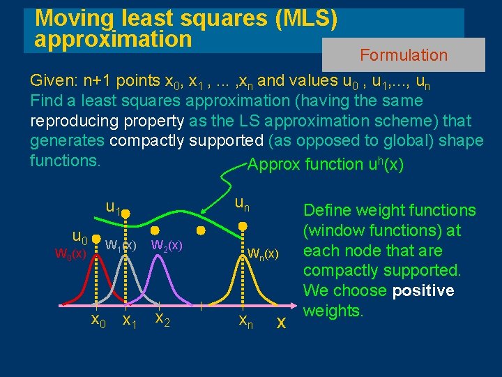
Moving least squares (MLS) approximation Formulation Given: n+1 points x 0, x 1 , . . . , xn and values u 0 , u 1, . . . , un Find a least squares approximation (having the same reproducing property as the LS approximation scheme) that generates compactly supported (as opposed to global) shape functions. Approx function uh(x) un u 1 u 0 W 0(x) W 1(x) x 0 x 1 W 2(x) x 2 Wn(x) xn x Define weight functions (window functions) at each node that are compactly supported. We choose positive weights.

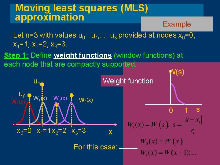
Moving least squares (MLS) approximation Example Let n=3 with values u 0 , u 1, . . . , u 3 provided at nodes x 0=0, x 1=1, x 2=2, x 3=3. Step 1: Define weight functions (window functions) at each node that are compactly supported. W(s) u 1 Weight function u 0 W 0(x) W 1(x) W 2(x) W 3(x) 0 x 0=0 x 1=1 x 2=2 x 3=3 x For this case: 1 s

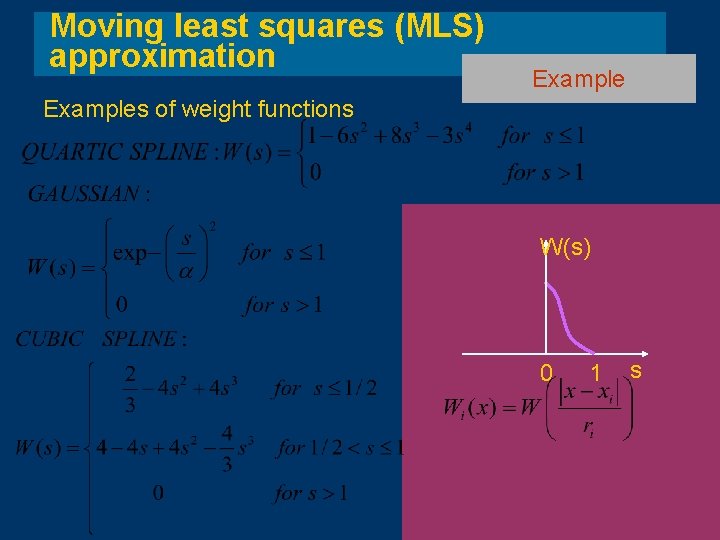
Moving least squares (MLS) approximation Examples of weight functions W(s) 0 1 s

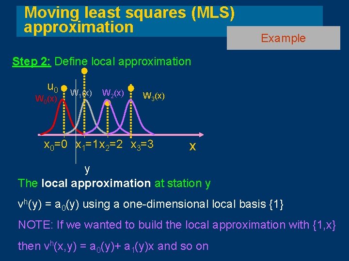
Moving least squares (MLS) approximation Example Step 2: Define local approximation u 0 W 0(x) W 1(x) W 2(x) W 3(x) x 0=0 x 1=1 x 2=2 x 3=3 x y The local approximation at station y vh(y) = a 0(y) using a one-dimensional local basis {1} NOTE: If we wanted to build the local approximation with {1, x} then vh(x, y) = a 0(y)+ a 1(y)x and so on

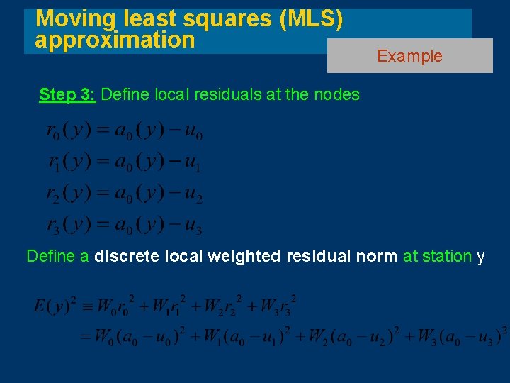
Moving least squares (MLS) approximation Example Step 3: Define local residuals at the nodes Define a discrete local weighted residual norm at station y

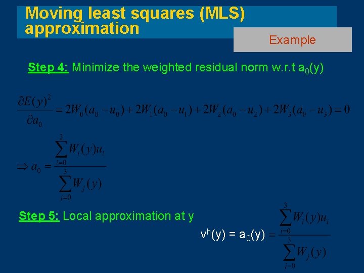
Moving least squares (MLS) approximation Example Step 4: Minimize the weighted residual norm w. r. t a 0(y) Step 5: Local approximation at y vh(y) = a 0(y)

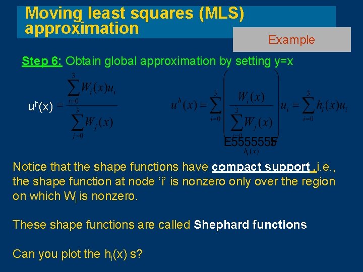
Moving least squares (MLS) approximation Example Step 6: Obtain global approximation by setting y=x uh(x) Notice that the shape functions have compact support , i. e. , the shape function at node ‘i’ is nonzero only over the region on which Wi is nonzero. These shape functions are called Shephard functions Can you plot the hi(x) s?

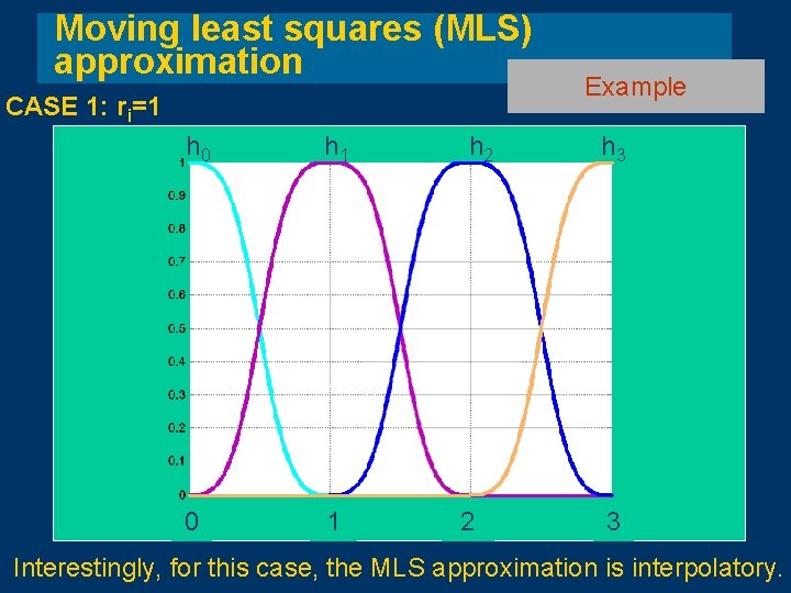
Moving least squares (MLS) approximation CASE 1: ri=1 h 0 h 1 0 1 h 2 2 Example h 3 3 Interestingly, for this case, the MLS approximation is interpolatory.

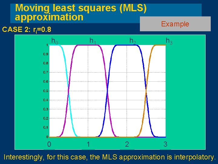
Moving least squares (MLS) approximation CASE 2: ri=0. 8 h 0 0 h 1 1 h 2 2 Example h 3 3 Interestingly, for this case, the MLS approximation is interpolatory.

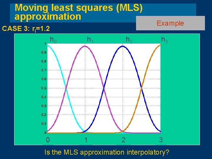
Moving least squares (MLS) approximation CASE 3: ri=1. 2 h 0 0 h 1 1 h 2 2 Example h 3 3 Is the MLS approximation interpolatory?

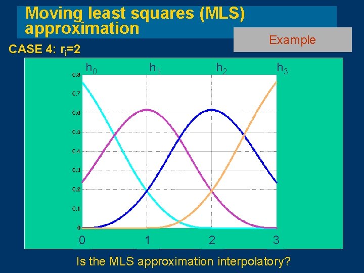
Moving least squares (MLS) approximation CASE 4: ri=2 h 0 0 h 1 1 h 2 2 Example h 3 3 Is the MLS approximation interpolatory?

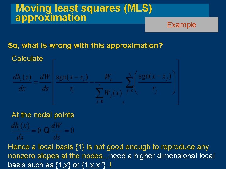
Moving least squares (MLS) approximation h 0 h 1 h 2 So, what is wrong with this approximation? Example h 3 Calculate At the nodal points Hence a local basis {1} is not good enough to reproduce any nonzero slopes at the nodes. . . need a higher dimensional local basis such as {1, x} or {1, x, x 2}. . !

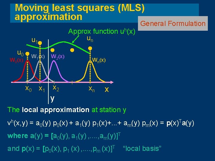
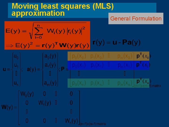
Moving least squares (MLS) approximation Approx function uh(x) un u 1 u 0 W 0(x) W 1(x) x 0 x 1 W 2(x) x 2 y General Formulation Wn(x) xn x The local approximation at station y vh(x, y) = a 0(y) p 0(x) + a 1(y) p 1(x)+. . . + am(y) pm(x) = p(x)Ta(y) where a(y) = [a 0(y), a 1(y) , . . , am(y)]T and p(x) = [p 0(x), p 1 (x) , . . , pm (x)]T “local basis”

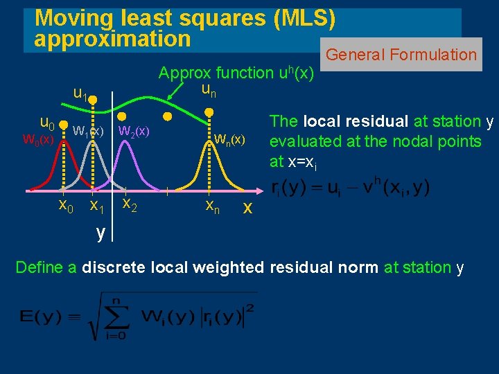
Moving least squares (MLS) approximation Approx function uh(x) un u 1 u 0 W 0(x) W 1(x) x 0 x 1 W 2(x) x 2 Wn(x) xn General Formulation The local residual at station y evaluated at the nodal points at x=xi x y Define a discrete local weighted residual norm at station y

Moving least squares (MLS) approximation General Formulation

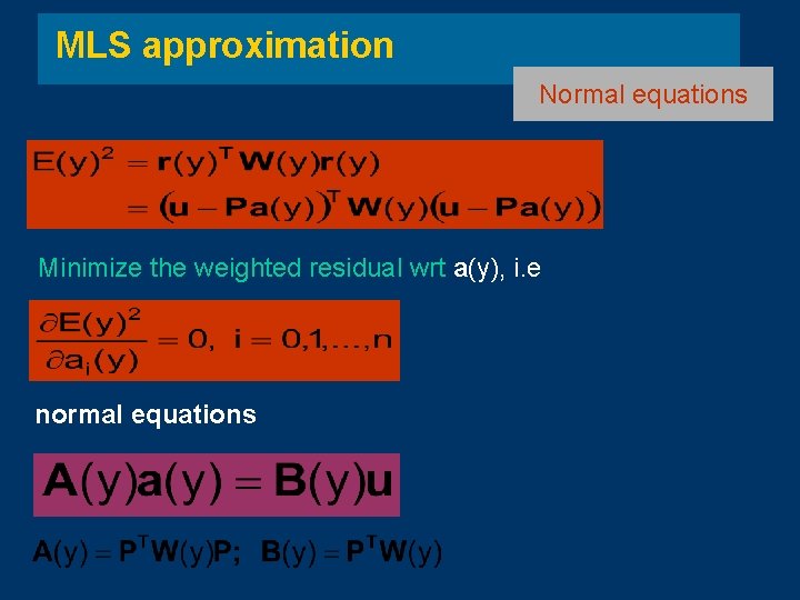
MLS approximation Normal equations Minimize the weighted residual wrt a(y), i. e normal equations

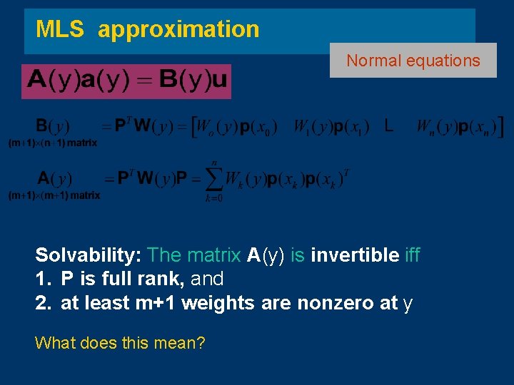
MLS approximation Normal equations Solvability: The matrix A(y) is invertible iff 1. P is full rank, and 2. at least m+1 weights are nonzero at y What does this mean?

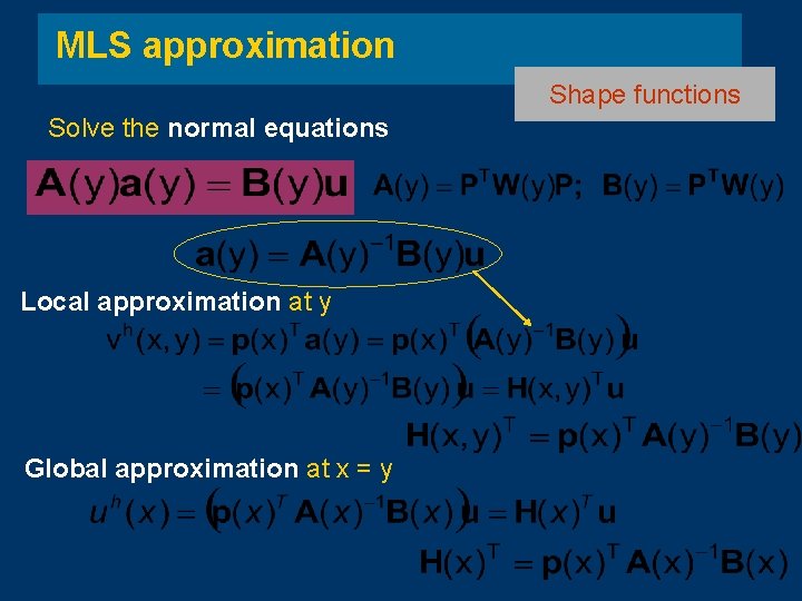
MLS approximation Shape functions Solve the normal equations Local approximation at y Global approximation at x = y

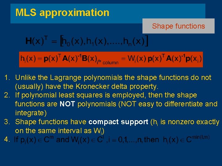
MLS approximation Shape functions 1. Unlike the Lagrange polynomials the shape functions do not (usually) have the Kronecker delta property. 2. If polynomial least squares is employed, then the shape functions are NOT polynomials (NOT easy to differentiate and integrate) 3. Shape functions have compact support (hi is nonzero exactly on the same interval as Wi) 4.

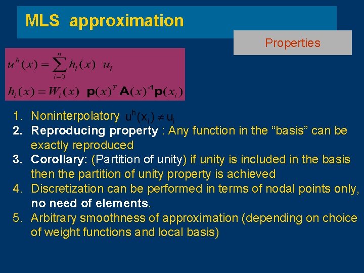
MLS approximation Properties 1. Noninterpolatory 2. Reproducing property : Any function in the “basis” can be exactly reproduced 3. Corollary: (Partition of unity) if unity is included in the basis then the partition of unity property is achieved 4. Discretization can be performed in terms of nodal points only, no need of elements. 5. Arbitrary smoothness of approximation (depending on choice of weight functions and local basis)

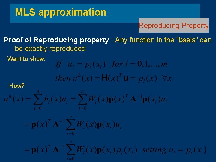
MLS approximation Reproducing Property Proof of Reproducing property : Any function in the “basis” can be exactly reproduced Want to show: How?

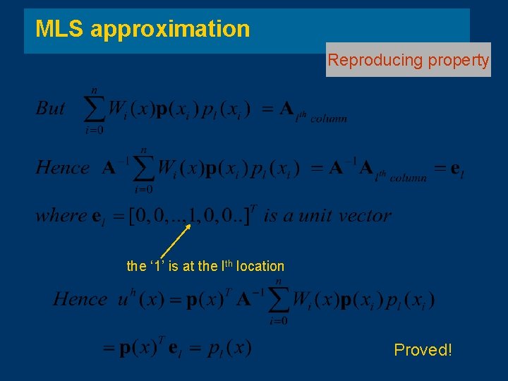
MLS approximation Reproducing property the ‘ 1’ is at the lth location Proved!

Shepard functions Consider the simplest case p(x) = [1] Shepard function 1. Reproducing property : Can reproduce constant functions only (rigid body modes) 2. Noninterpolatory. However, if special (singular) weights are chosen these functions can interpolate the data (IMLS)

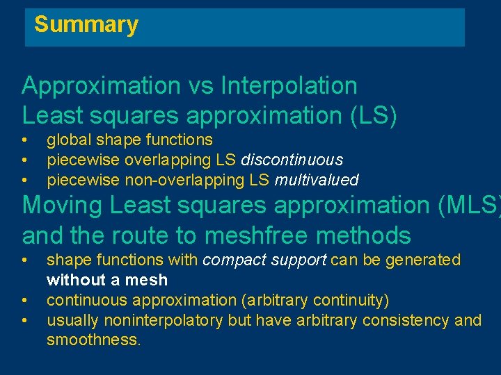
Summary Approximation vs Interpolation Least squares approximation (LS) • • • global shape functions piecewise overlapping LS discontinuous piecewise non-overlapping LS multivalued Moving Least squares approximation (MLS) and the route to meshfree methods • • • shape functions with compact support can be generated without a mesh continuous approximation (arbitrary continuity) usually noninterpolatory but have arbitrary consistency and smoothness.

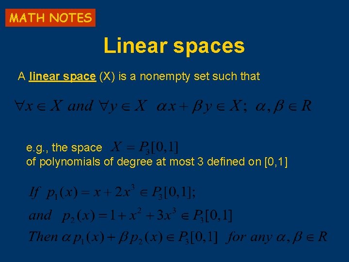
MATH NOTES Linear spaces A linear space (X) is a nonempty set such that e. g. , the space of polynomials of degree at most 3 defined on [0, 1]

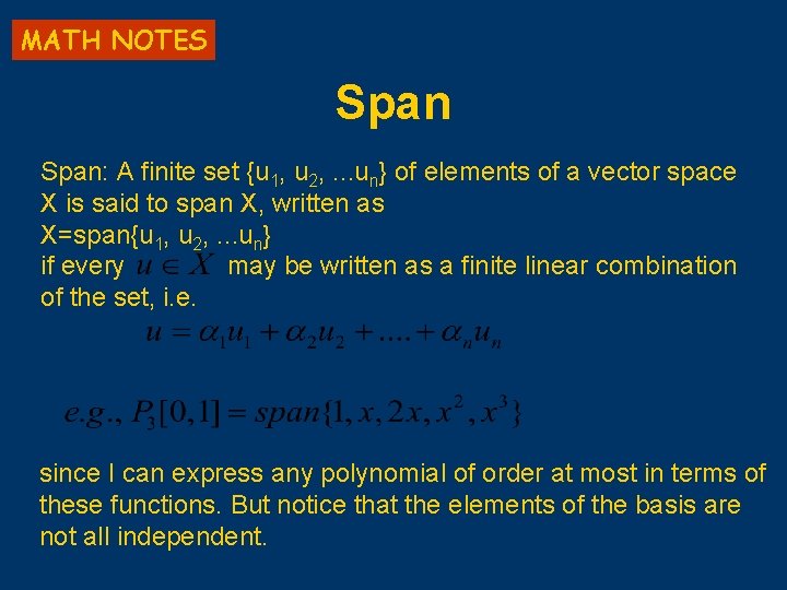
MATH NOTES Span: A finite set {u 1, u 2, . . . un} of elements of a vector space X is said to span X, written as X=span{u 1, u 2, . . . un} if every may be written as a finite linear combination of the set, i. e. since I can express any polynomial of order at most in terms of these functions. But notice that the elements of the basis are not all independent.

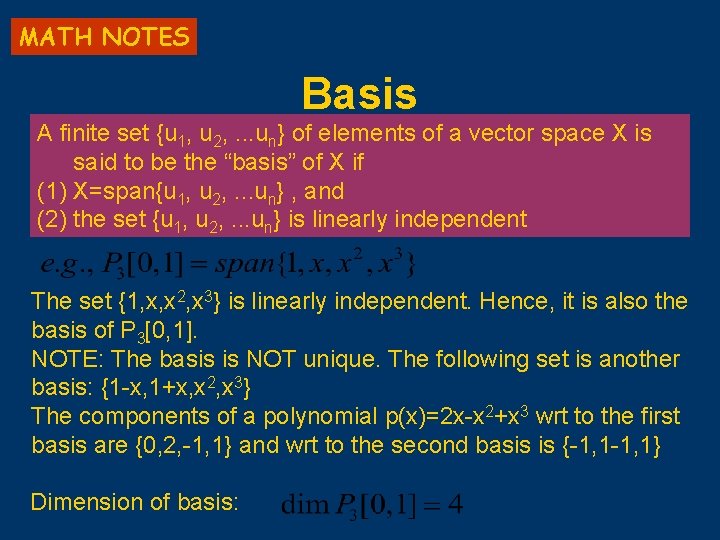
MATH NOTES Basis A finite set {u 1, u 2, . . . un} of elements of a vector space X is said to be the “basis” of X if (1) X=span{u 1, u 2, . . . un} , and (2) the set {u 1, u 2, . . . un} is linearly independent The set {1, x, x 2, x 3} is linearly independent. Hence, it is also the basis of P 3[0, 1]. NOTE: The basis is NOT unique. The following set is another basis: {1 -x, 1+x, x 2, x 3} The components of a polynomial p(x)=2 x-x 2+x 3 wrt to the first basis are {0, 2, -1, 1} and wrt to the second basis is {-1, 1} Dimension of basis: