Generalizations of Filter Bank Analyzer Signal preprocessor conditions

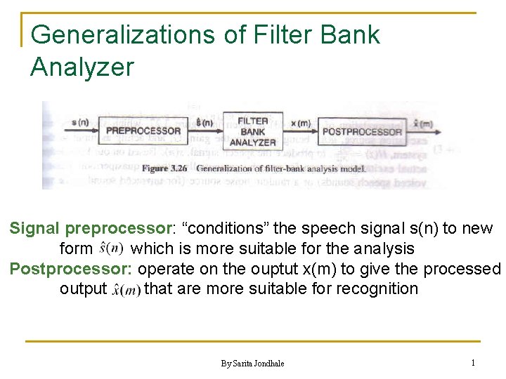
Generalizations of Filter Bank Analyzer Signal preprocessor: “conditions” the speech signal s(n) to new form which is more suitable for the analysis Postprocessor: operate on the ouptut x(m) to give the processed output that are more suitable for recognition By Sarita Jondhale 1

Generalizations of Filter Bank Analyzer Preprocessor Operations n n n Signal preemphasis: higher frequencies are increased in amplitude Noise elimination Signal enhancement (to make the formant peaks more prominent) The purpose of pre processor is to make the speech signal as clean as possible By Sarita Jondhale 2

Generalizations of Filter Bank Analyzer Postprocessor Operations n n n sp Temporal smoothing of sequential filter bank output vectors. Frequency smoothing of individual filter bank output vectors. Normalization of each filter bank output vector Thresholding and/or quantization of the filter-bank outputs vectors Principal components analysis of the filter bank output vector. The purpose of postprocessor is to clean up the output so as to best represent the spectral information in the speech signal. By Sarita Jondhale 3

Spectral Analysis n Two methods: q The Filter Bank spectrum q The Linear Predictive coding (LPC) By Sarita Jondhale 4

Linear Predictive Coding Estimating the parameters of the current speech sample by using the parameter values from linear combinations of past speech samples. By Sarita Jondhale 5

n n Linear Predictive Coding (or “LPC”) is a method of predicting a sample of a speech signal based on several previous samples. We can use the LPC coefficients to separate a speech signal into two parts: the transfer function (which contains the vocal quality) and the excitation (which contains the pitch and the sound). By Sarita Jondhale 8

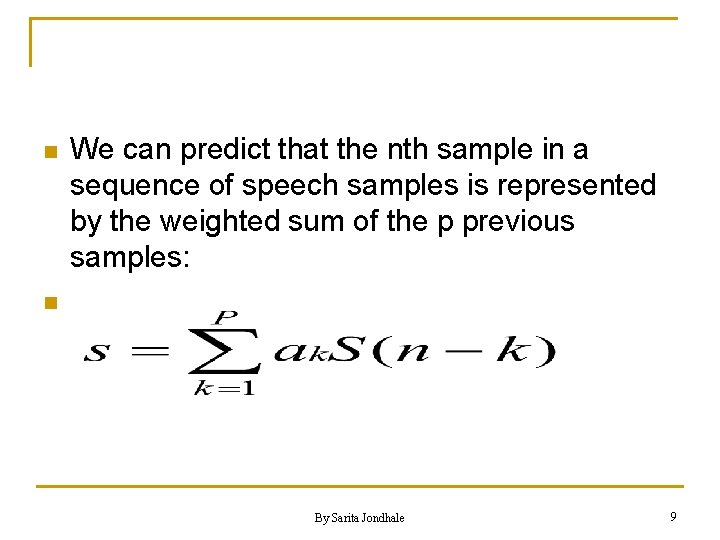
n We can predict that the nth sample in a sequence of speech samples is represented by the weighted sum of the p previous samples: n By Sarita Jondhale 9

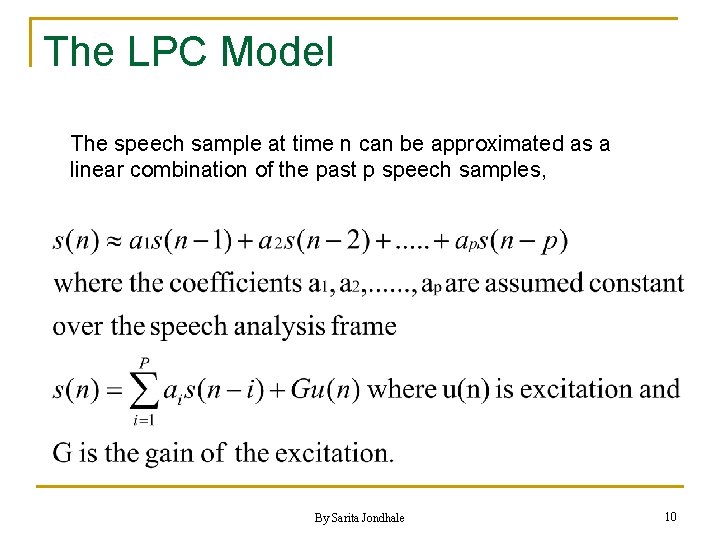
The LPC Model The speech sample at time n can be approximated as a linear combination of the past p speech samples, By Sarita Jondhale 10

n n n The number of samples (p) is referred to as the “order” of the LPC. As p approaches infinity, we should be able to predict the nth sample exactly. However, p is usually on the order of ten to twenty, where it can provide an accurate enough representation with a limited cost of computation. The weights on the previous samples (ak) are chosen in order to minimize the squared error between the real sample and its predicted value. Thus, we want the error signal e(n), which is sometimes referred to as the LPC residual, to be as small as possible By Sarita Jondhale 11

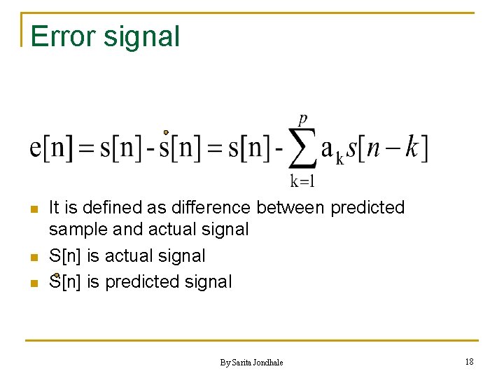
Error signal n n n It is defined as difference between predicted sample and actual signal S[n] is predicted signal By Sarita Jondhale 18

LPC Analysis Equations n Two methods of defining the range of speech (m) q q The autocorrelation method The covariance method By Sarita Jondhale 25

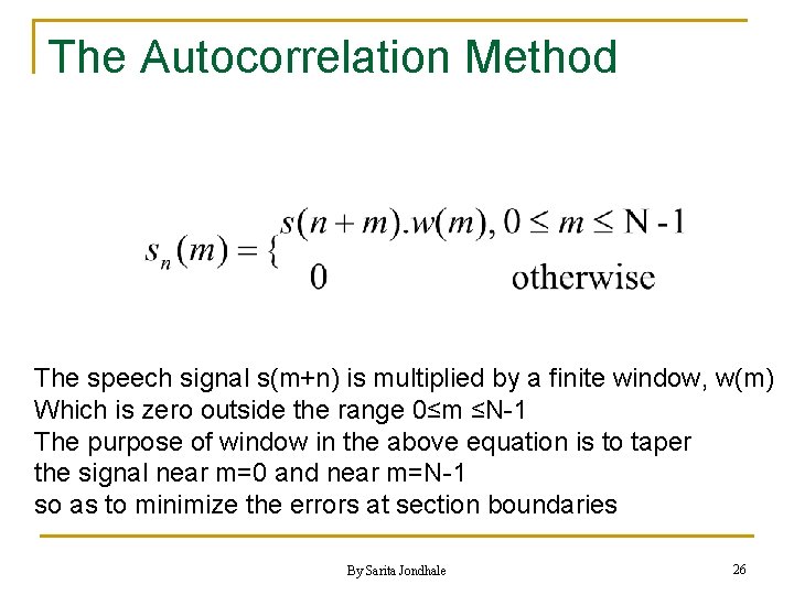
The Autocorrelation Method The speech signal s(m+n) is multiplied by a finite window, w(m) Which is zero outside the range 0≤m ≤N-1 The purpose of window in the above equation is to taper the signal near m=0 and near m=N-1 so as to minimize the errors at section boundaries By Sarita Jondhale 26

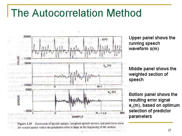
The Autocorrelation Method Upper panel shows the running speech waveform s(m) Middle panel shows the weighted section of speech Bottom panel shows the resulting error signal en(m), based on optimum selection of predictor parameters By Sarita Jondhale 27

The Autocorrelation Method n n For m<0 , the prediction error i. e en(m)=0 since sn(m)=0 for all m<0 For m>N-1+p there is no prediction error because sn(m)=0 for all m>N-1 By Sarita Jondhale 30

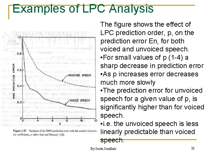
Examples of LPC Analysis The figure shows the effect of LPC prediction order, p, on the prediction error En, for both voiced and unvoiced speech. • For small values of p (1 -4) a sharp decrease in prediction error • As p increases error decreases much more slowly • The prediction error for unvoiced speech for a given value of p, is significantly higher than for voiced speech. • i. e. the unvoiced speech is less linearly predictable than voiced speech. By Sarita Jondhale 38

LPC Processor for Speech Recognition By Sarita Jondhale 40

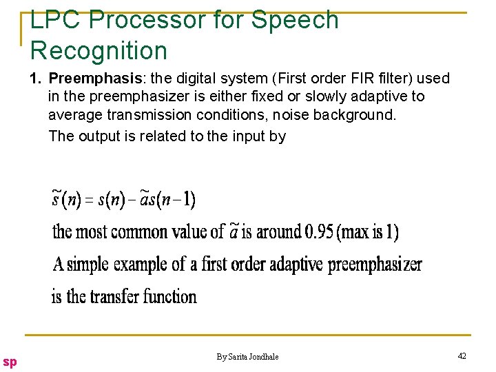
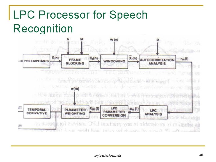
LPC Processor for Speech Recognition 1. Preemphasis: the digital system (First order FIR filter) used in the preemphasizer is either fixed or slowly adaptive to average transmission conditions, noise background. The output is related to the input by sp By Sarita Jondhale 42

LPC Processor for Speech Recognition 2. Frame Blocking: In this step the preemphasized speech signal is blocked into frames of N samples, with adjacent frames being separated by M samples. By Sarita Jondhale 43

Typical LPC Analysis Parameters n n n N: number of samples in analysis frame. M: number of samples shift between analysis frames. p: LPC analysis order. Q: dimension of LPC derived cepstral vector. K: number of frames over which cepstral time derivatives are computed. By Sarita Jondhale 44

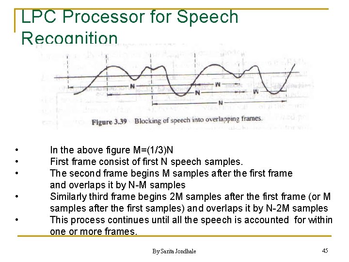
LPC Processor for Speech Recognition • • • In the above figure M=(1/3)N First frame consist of first N speech samples. The second frame begins M samples after the first frame and overlaps it by N-M samples Similarly third frame begins 2 M samples after the first frame (or M samples after the first samples) and overlaps it by N-2 M samples This process continues until all the speech is accounted for within one or more frames. By Sarita Jondhale 45

LPC Processor for Speech Recognition By Sarita Jondhale 46

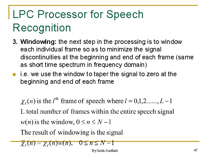
LPC Processor for Speech Recognition 3. Windowing: the next step in the processing is to window each individual frame so as to minimize the signal discontinuities at the beginning and end of each frame (same as short time spectrum in frequency domain) n i. e. we use the window to taper the signal to zero at the beginning and end of each frame By Sarita Jondhale 47

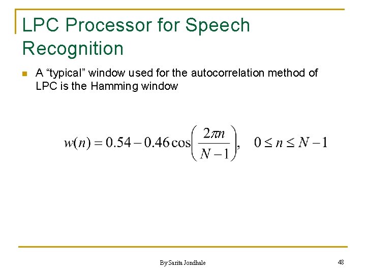
LPC Processor for Speech Recognition n A “typical” window used for the autocorrelation method of LPC is the Hamming window By Sarita Jondhale 48

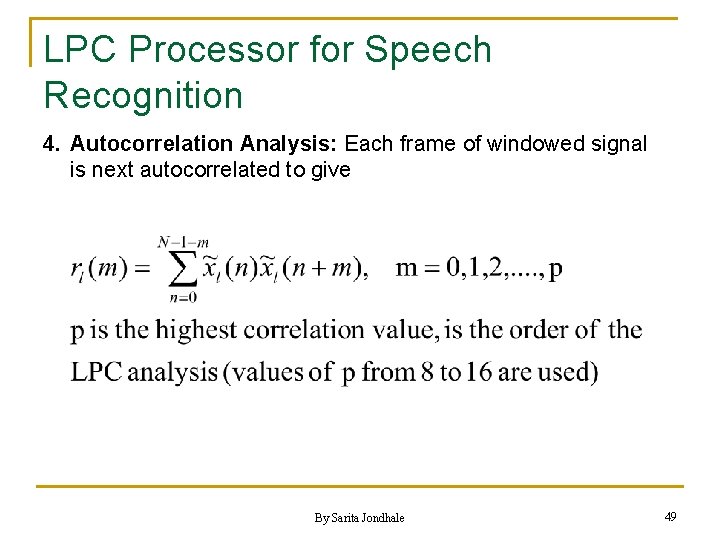
LPC Processor for Speech Recognition 4. Autocorrelation Analysis: Each frame of windowed signal is next autocorrelated to give By Sarita Jondhale 49

LPC Processor for Speech Recognition 5. LPC Analysis: the next step is the LPC analysis, which converts each frame of P+1 autocorrelations into an “LPC parameter set”. n The set might be q The LPC coefficients q The reflection (or PARCOR) coefficients q The log area ratio coefficients q The cepstral coefficients q Or any desired transformations of the above sets n The method for converting from autocorrelation coefficients to an LPC parameter set is known as Durbin’s method By Sarita Jondhale 50

LPC Processor for Speech Recognition n n The cepstral coefficients are the coefficients of the FT representation of the log magnitude spectrum. The cepstral coefficients are more robust reliable feature set for speech recognition than the LPC coefficients, the PARCOR coefficients, or the log area ratio coefficients. By Sarita Jondhale 53

LPC Processor for Speech Recognition 7. Parameter Weighting: because of the sensitivity of the loworder cepstral coefficients to overall spectral slope and sensitivity of the high-order cepstral coefficients to noise, it is necessary to weight the cepstral coefficients by a tapered window to minimize these sensitivities. By Sarita Jondhale 54

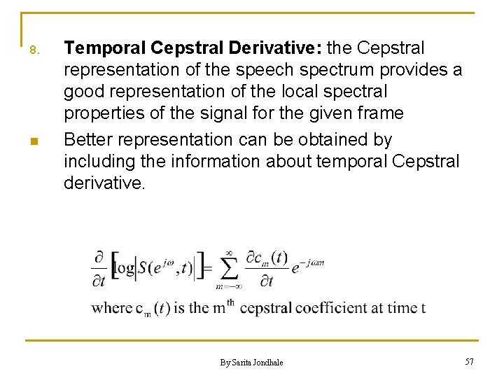
8. n Temporal Cepstral Derivative: the Cepstral representation of the speech spectrum provides a good representation of the local spectral properties of the signal for the given frame Better representation can be obtained by including the information about temporal Cepstral derivative. By Sarita Jondhale 57