General Linear Model With correlated error terms S

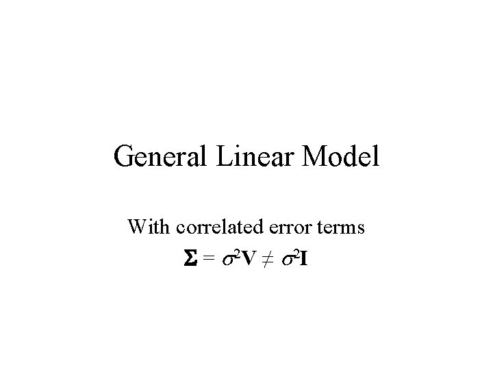
General Linear Model With correlated error terms S = s 2 V ≠ s 2 I

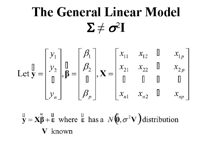
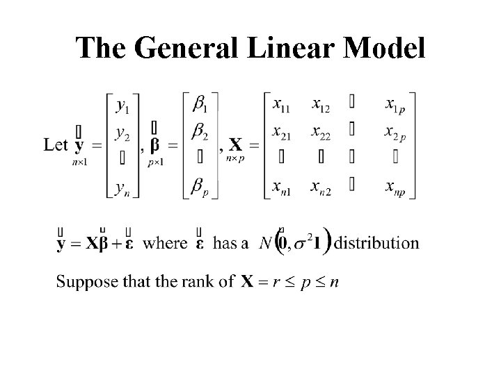
The General Linear Model S ≠ s 2 I

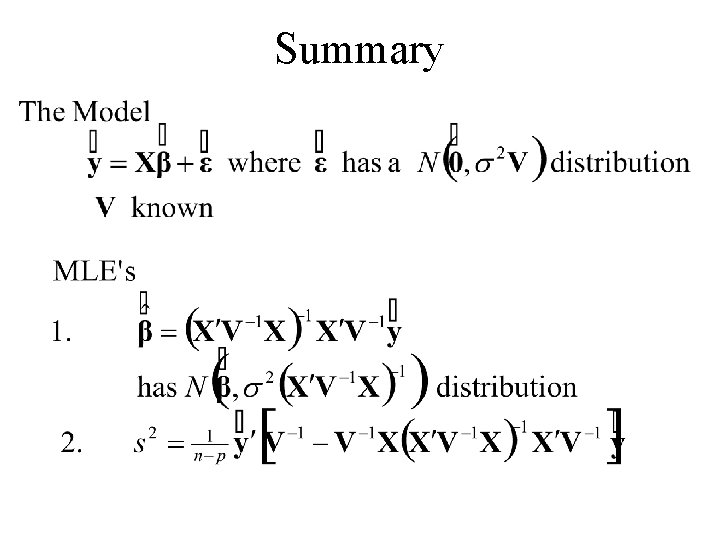
Summary

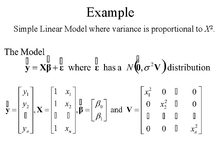
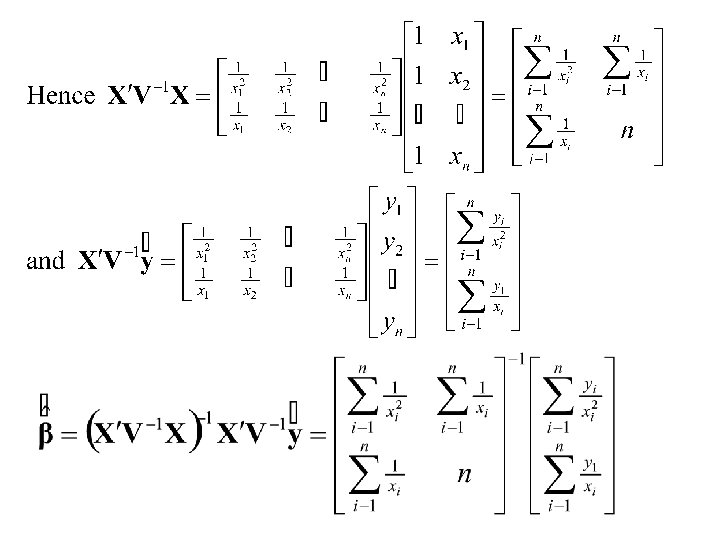
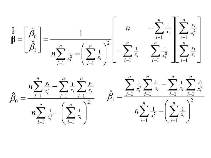
Example Simple Linear Model where variance is proportional to X 2.

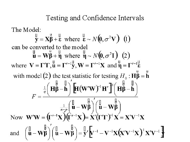
Testing and Confidence Intervals The Model: can be converted to the model

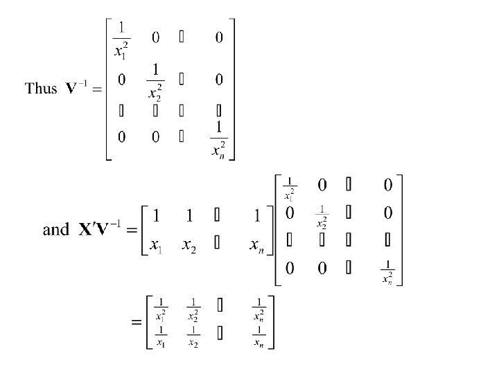
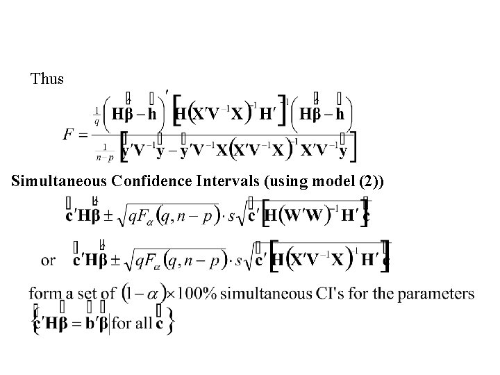
Thus Simultaneous Confidence Intervals (using model (2))

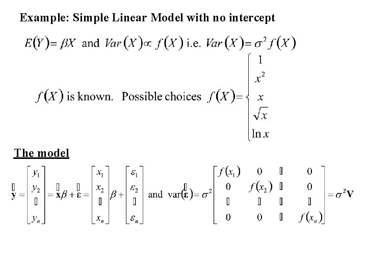
Example: Simple Linear Model with no intercept The model

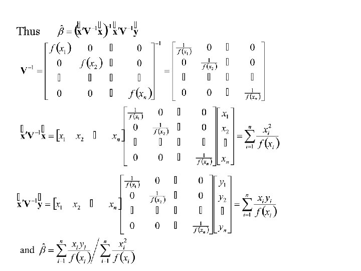
Thus

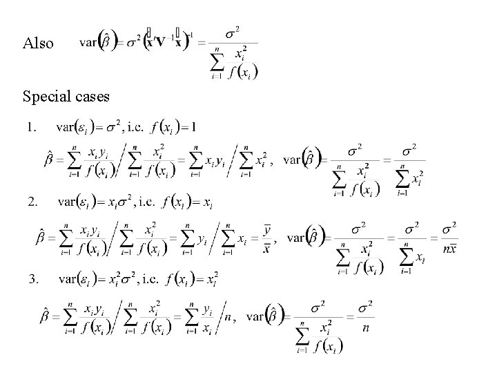
Also Special cases

General Linear Model Case 2: S unknown

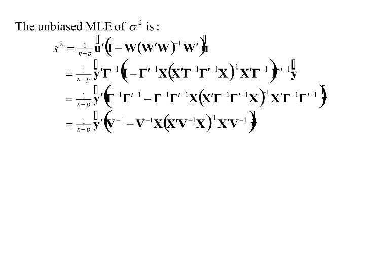
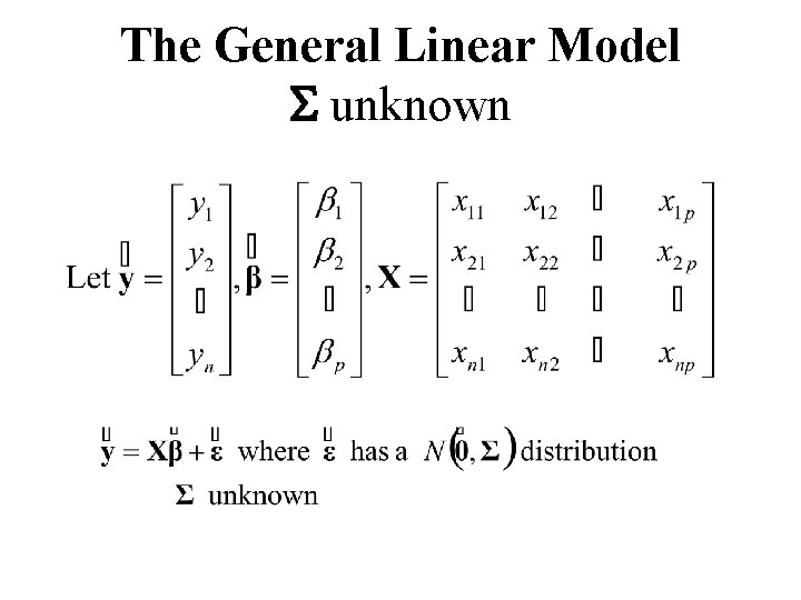
The General Linear Model S unknown

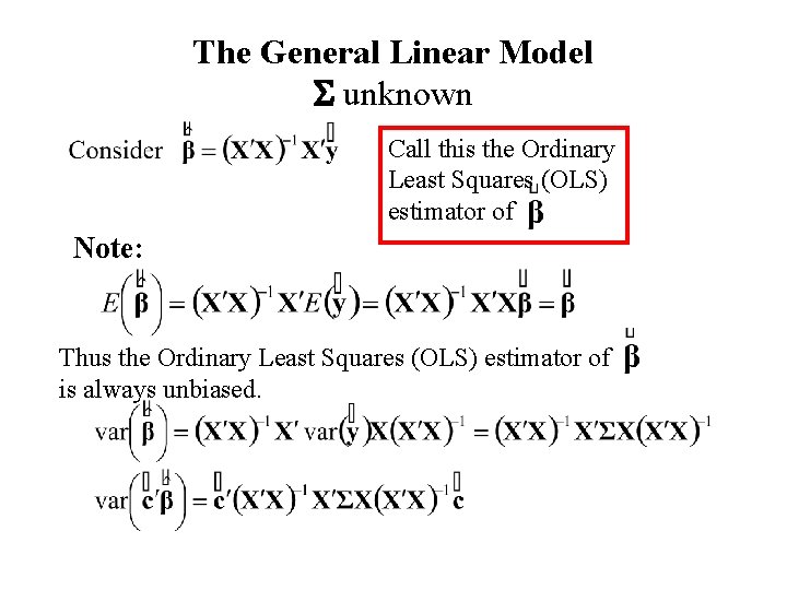
The General Linear Model S unknown Call this the Ordinary Least Squares (OLS) estimator of Note: Thus the Ordinary Least Squares (OLS) estimator of is always unbiased.

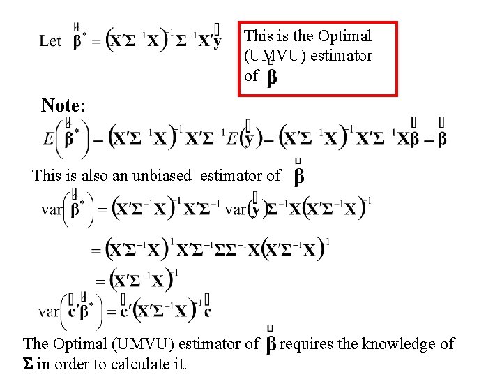
This is the Optimal (UMVU) estimator of Note: This is also an unbiased estimator of The Optimal (UMVU) estimator of S in order to calculate it. requires the knowledge of

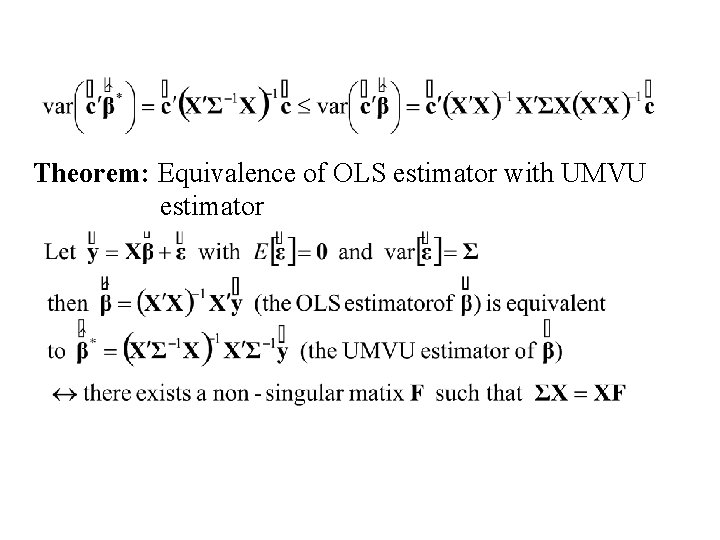
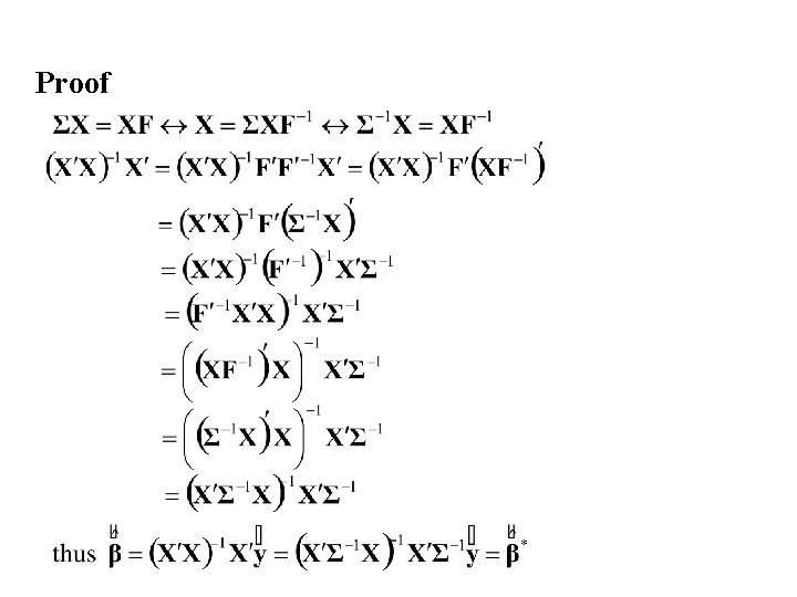
Theorem: Equivalence of OLS estimator with UMVU estimator

Proof

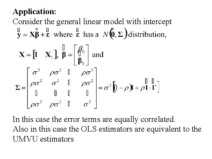
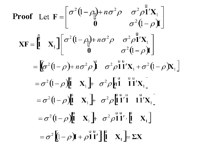
Application: Consider the general linear model with intercept In this case the error terms are equally correlated. Also in this case the OLS estimators are equivalent to the UMVU estimators

Proof

Design Matrix, X, not of full rank

The General Linear Model

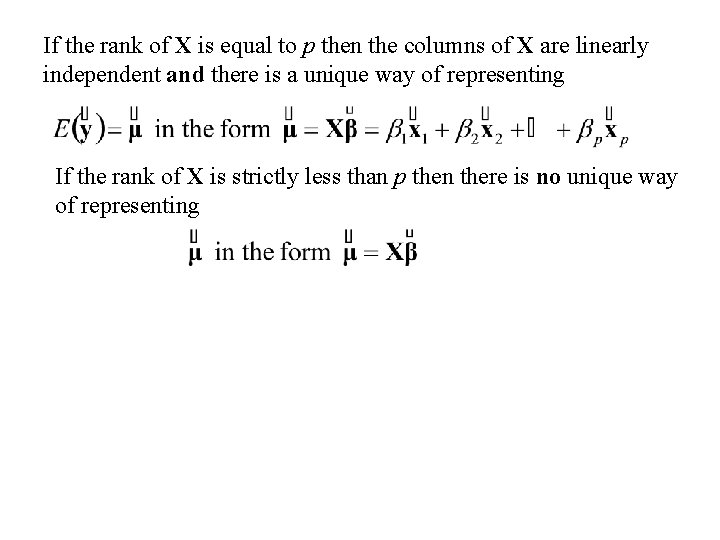
If the rank of X is equal to p then the columns of X are linearly independent and there is a unique way of representing If the rank of X is strictly less than p then there is no unique way of representing

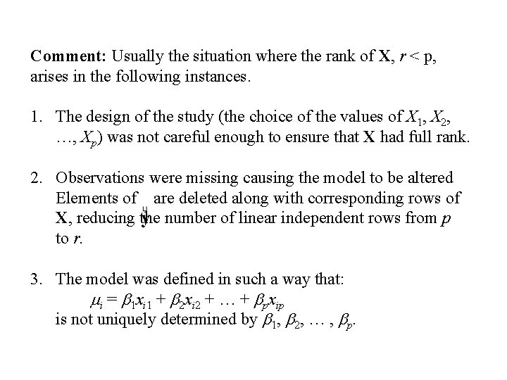
Comment: Usually the situation where the rank of X, r < p, arises in the following instances. 1. The design of the study (the choice of the values of X 1, X 2, …, Xp) was not careful enough to ensure that X had full rank. 2. Observations were missing causing the model to be altered Elements of are deleted along with corresponding rows of X, reducing the number of linear independent rows from p to r. 3. The model was defined in such a way that: mi = b 1 xi 1 + b 2 xi 2 + … + bpxip is not uniquely determined by b 1, b 2, … , bp.

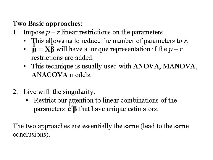
Two Basic approaches: 1. Impose p – r linear restrictions on the parameters • This allows us to reduce the number of parameters to r. • will have a unique representation if the p – r restrictions are added. • This technique is usually used with ANOVA, MANOVA, ANACOVA models. 2. Live with the singularity. • Restrict our attention to linear combinations of the parameters that have unique estimators. The two approaches are essentially the same (lead to the same conclusions).

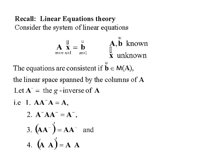
Recall: Linear Equations theory Consider the system of linear equations M(A), the linear space spanned by the columns of A

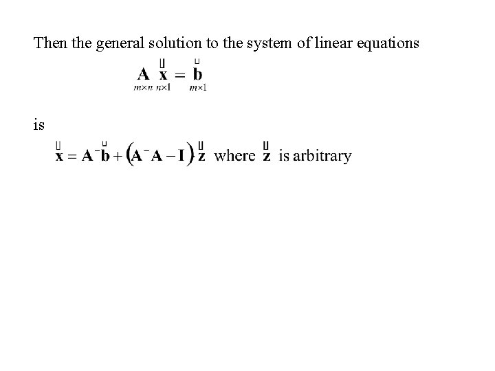
Then the general solution to the system of linear equations is

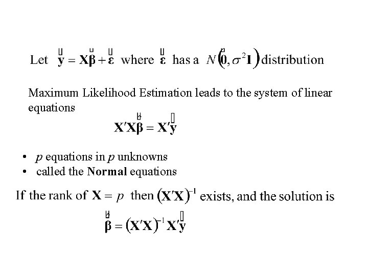
Maximum Likelihood Estimation leads to the system of linear equations • p equations in p unknowns • called the Normal equations

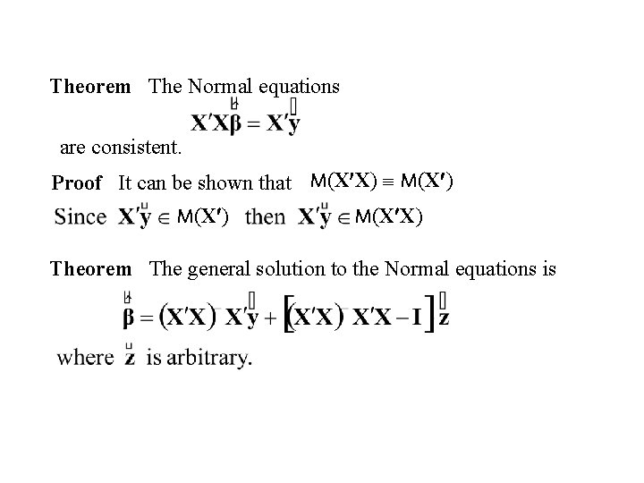
Theorem The Normal equations are consistent. Proof It can be shown that M(X X) M(X ) M(X X) Theorem The general solution to the Normal equations is

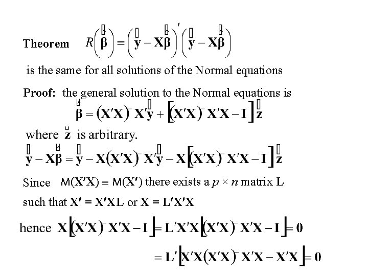
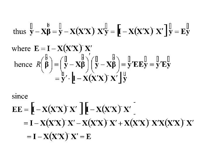
Theorem is the same for all solutions of the Normal equations Proof: the general solution to the Normal equations is Since M(X X) M(X ) there exists a p × n matrix L such that X = X XL or X = L X X

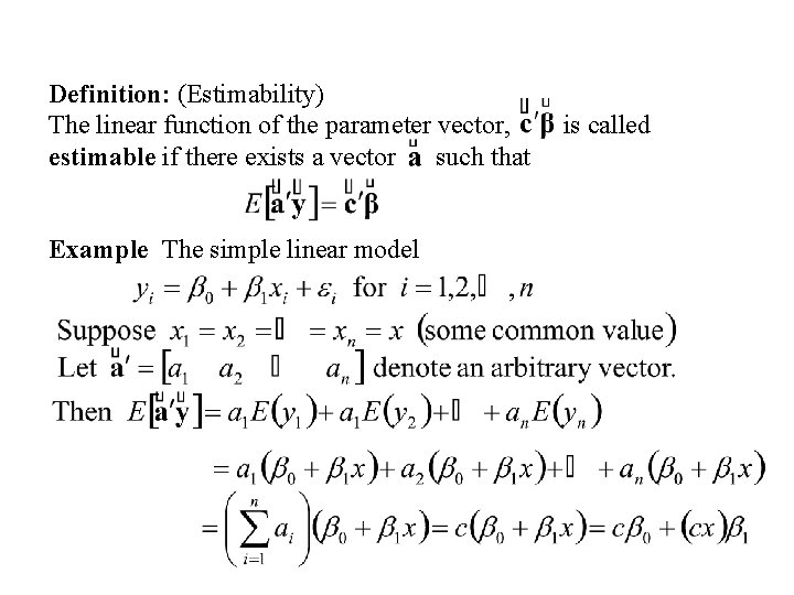
Definition: (Estimability) The linear function of the parameter vector, estimable if there exists a vector such that Example The simple linear model is called

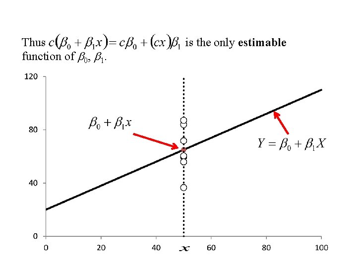
Thus function of b 0, b 1. is the only estimable

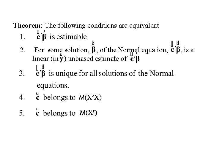
Theorem: The following conditions are equivalent 2. For some solution, , of the Normal equation, linear (in ) unbiased estimate of M(X X) M(X ) , is a

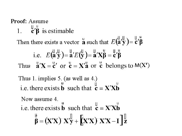
Proof: Assume Then there exists a vector such that Thus 1. implies 5. (as well as 4. ) Now assume 4. M(X )

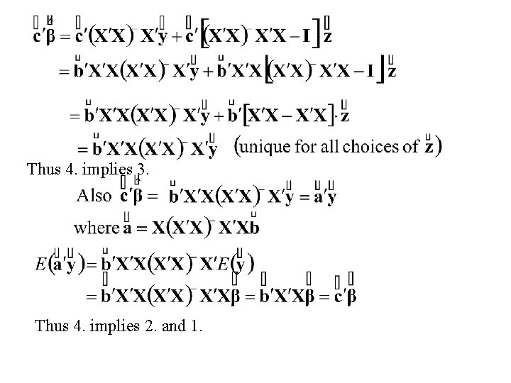
Thus 4. implies 3. Thus 4. implies 2. and 1.

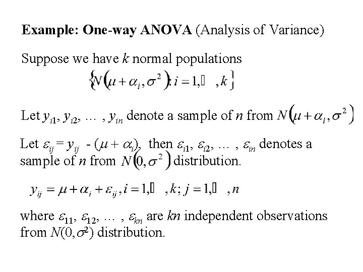
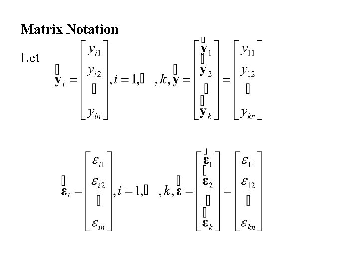
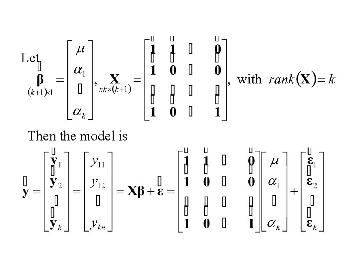
Example: One-way ANOVA (Analysis of Variance) Suppose we have k normal populations Let yi 1, yi 2, … , yin denote a sample of n from Let eij = yij - (m + ai), then ei 1, ei 2, … , ein denotes a sample of n from distribution. where e 11, e 12, … , ekn are kn independent observations from N(0, s 2) distribution.

Matrix Notation Let

Let Then the model is

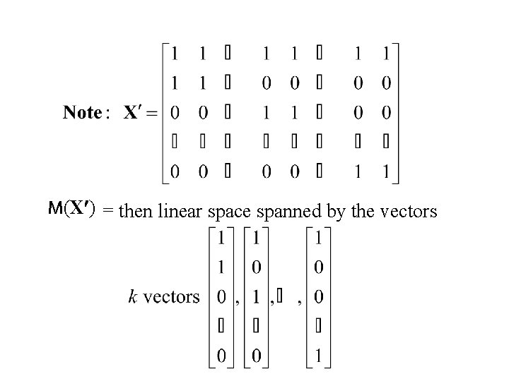
M(X ) = then linear space spanned by the vectors

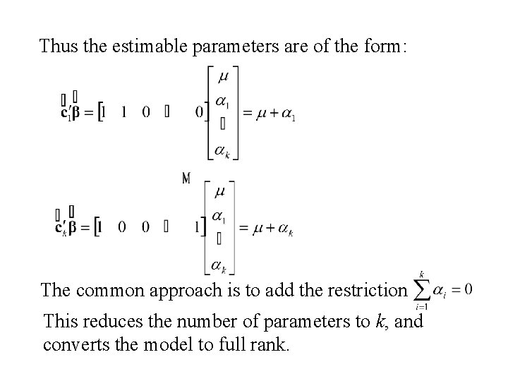
Thus the estimable parameters are of the form: The common approach is to add the restriction This reduces the number of parameters to k, and converts the model to full rank.

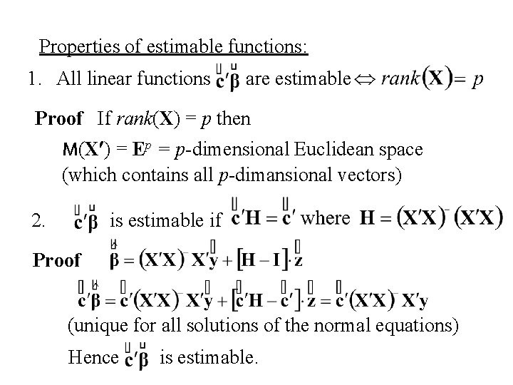
Properties of estimable functions: 1. All linear functions are estimable Proof If rank(X) = p then M(X ) = Ep = p-dimensional Euclidean space (which contains all p-dimansional vectors) 2. is estimable if Proof (unique for all solutions of the normal equations) Hence is estimable.

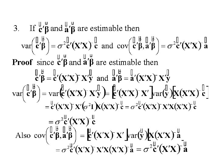
3. If and Proof since are estimable then and are estimable then