General additive models Variance and covariance Sums of

General additive models Variance and covariance Sums of squares M contains the mean

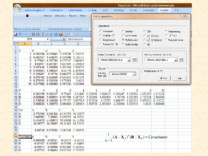
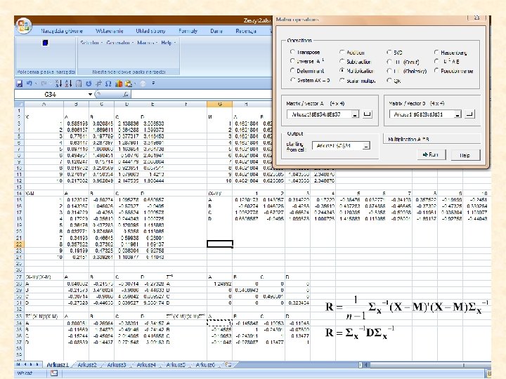
The coefficient of correlation We deal with samples For a matrix X that contains several variables holds The diagonal matrix SX contains the standard deviations as entries. X-M is called the central matrix. The matrix R is a symmetric distance matrix that contains all correlations between the variables

Pre-and postmultiplication Premultiplication Postmultiplication For diagonal matrices X holds

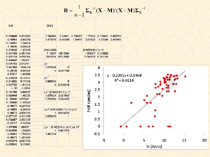
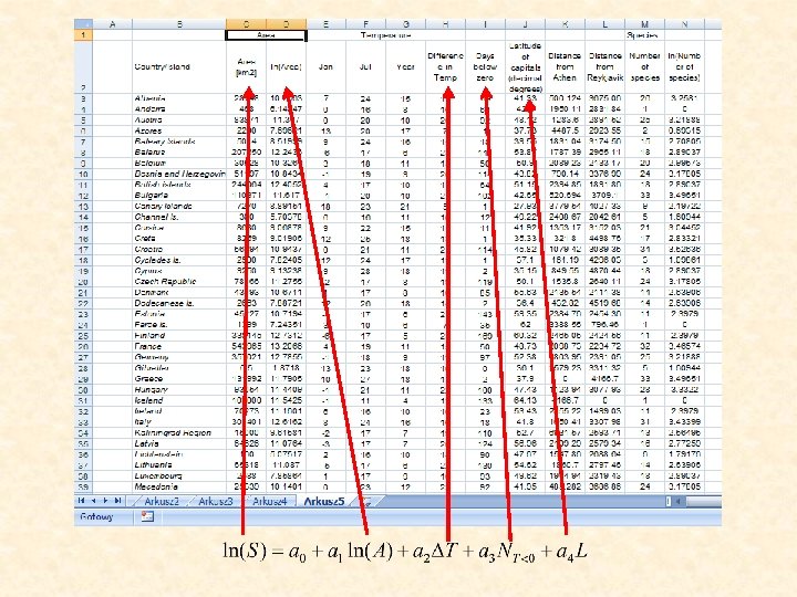
Linear regression European bat species and environmental correlates

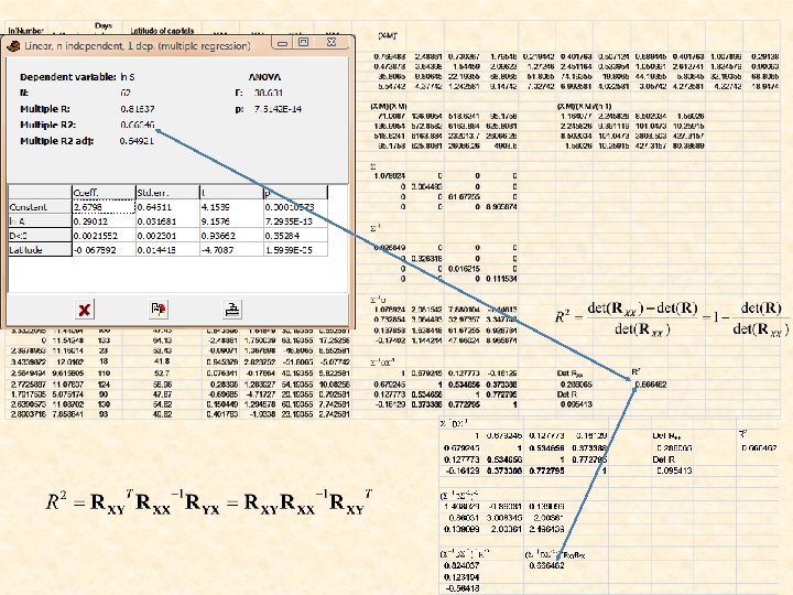
N=62 Matrix approach to linear regression X is not a square matrix, hence X-1 doesn’t exist.

The species – area relationship of European bats What about the part of variance explained by our model? 1. 16: Average number of species per unit area (species density) 0. 24: spatial species turnover

How to interpret the coefficient of determination Total variance Rest (unexplained) variance Residual (explained) variance Statistical testing is done by an F or a t-test.

The general linear model A model that assumes that a dependent variable Y can be expressed by a linear combination of predictor variables X is called a linear model. The vector E contains the error terms of each regression. Aim is to minimize E.

The general linear model If the errors of the preictor variables are Gaussian the error term e should also be Gaussian and means and variances are additive Total variance Explained variance Unexplained (rest) variance

Multiple regression 1. Model formulation 2. Estimation of model parameters 3. Estimation of statistical significance

Multiple R and R 2

The coefficient of determination y x 1 x 2 xm The correlation matrix can be devided into four compartments.

R: correlation matrix n: number of cases k: number of independent variables in the model D<0 is statistically not significant and should be eliminated from the model. Adjusted R 2

A mixed model

The final model Negative species density Realistic increase of species richness with area Increase of species richness with winter length Increase of species richness at higher latitudes A peak of species richness at intermediate latitudes Is this model realistic? The model makes a series of unrealistic predictions. Our initial assumptions are wrong despite of the high degree of variance explanation Our problem arises in part from the intercorrelation between the predictor variables (multicollinearity). We solve the problem by a stepwise approach eliminating the variables that are either not significant or give unreasonable parameter values The variance explanation of this final model is higher than that of the previous one.

Multiple regression solves systems of intrinsically linear algebraic equations Polynomial regression • • • General additive model The matrix X’X must not be singular. It est, the variables have to be independent. Otherwise we speak of multicollinearity. Collinearity of r<0. 7 are in most cases tolerable. Multiple regression to be safely applied needs at least 10 times the number of cases than variables in the model. Statistical inference assumes that errors have a normal distribution around the mean. The model assumes linear (or algebraic) dependencies. Check first for non-linearities. Check the distribution of residuals Yexp-Yobs. This distribution should be random. Check the parameters whether they have realistic values. Multiple regression is a hypothesis testing and not a hypothesis generating technique!!

Standardized coefficients of correlation Z-tranformed distributions have a mean of 0 an a standard deviation of 1. In the case of bivariate regression Y = a. X+b, Rxx = 1. Hence B=RXY. Hence the use of Z-transformed values results in standardized correlations coefficients, termed b-values

How to interpret beta-values If then Beta values are generalisations of simple coefficients of correlation. However, there is an important difference. The higher the correlation between two or more predicator variables (multicollinearity) is, the less will r depend on the correlation between X and Y. Hence other variables might have more and more influence on r and b. For high levels of multicollinearity it might therefore become more and more difficult to interpret beta-values in terms of correlations. Because beta-values are standardized b-values they should allow comparisons to be make about the relative influence of predicator variables. High levels of multicollinearity might let to misinterpretations. Beta values above one are always a sign of too high multicollinearity Hence high levels of multicollinearity might · reduce the exactness of beta-weight estimates · change the probabilities of making type I and type II errors · make it more difficult to interpret beta-values. We might apply an additional parameter, the so-called coefficient of structure. The coefficient of structure ci is defined as where ri. Y denotes the simple correlation between predicator variable i and the dependent variable Y and R 2 the coefficient of determination of the multiple regression. Coefficients of structure measure therefore the fraction of total variability a given predictor variable explains. Again, the interpretation of ci is not always unequivocal at high levels of multicollinearity.

Partial correlations The partial correlation rxy/z is the correlation of the residuals DX and DY Semipartial correlation A semipartial correlation correlates a variable with one residual only.

Path analysis and linear structure models Multiple regression The error term e contain the part of the variance in Y that is not explained by the model. These errors are called residuals Regression analysis does not study the relationships between the predictor variables Path analysis defines a whole model and tries to separate correlations into direct and indirect effects Path analysis tries to do something that is logically impossible, to derive causal relationships from sets of observations.

Path analysis is largely based on the computation of partial coefficients of correlation. Path coefficients Path analysis is a model confirmatory tool. It should not be used to generate models or even to seek for models that fit the data set. We start from regression functions

From Z-transformed values we get e. ZY = 0 ZYZY = 1 Path analysis is a nice tool to generate hypotheses. It fails at low coefficients of correlation and circular model structures. ZXZY = r. XY

Non-metric multiple regression

Statistical inference Rounding errors due to different precisions cause the residual variance to be larger than the total variance.

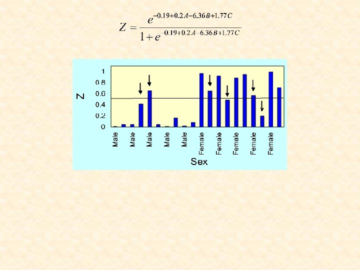
Logistic and other regression techniques We use odds The logistic regression model

Generalized non-linear regression models A special regression model that is used in pharmacology b 0 is the maximum response at dose saturation. b 1 is the concentration that produces a half maximum response. b 2 determines the slope of the function, that means it is a measure how fast the response increases with increasing drug dose.