Gene expression Clustering Chapter 10 Determining gene function

Gene expression & Clustering (Chapter 10)

Determining gene function • Sequence comparison tells us if a gene is similar to another gene, e. g. , in a new species – Dynamic programming – Approximate pattern matching • Genes with similar sequence likely to have similar function • Doesn’t always work. – “Homologous” genes may not be similar enough at the sequence level, to be detected this way • New method to determine gene function: directly measure gene activity (DNA arrays)

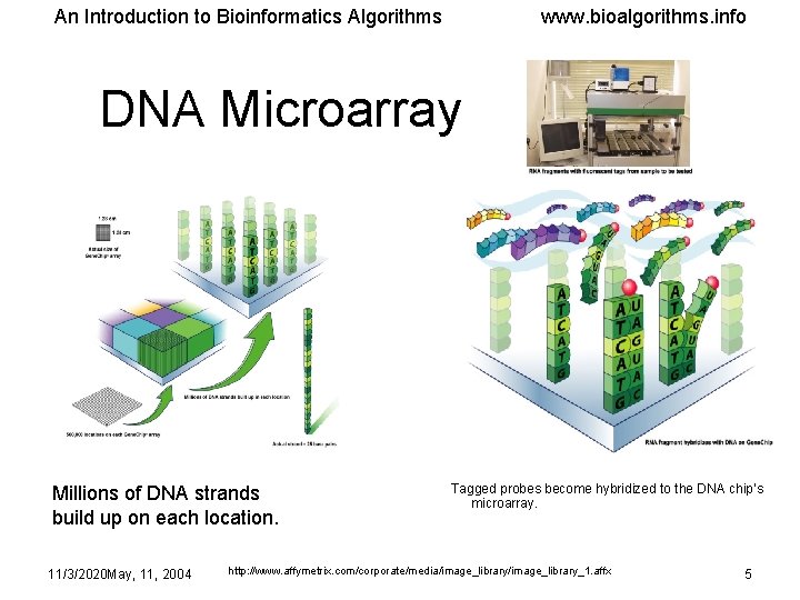
An Introduction to Bioinformatics Algorithms www. bioalgorithms. info DNA Arrays--Technical Foundations • An array works by exploiting the ability of a given m. RNA molecule to hybridize to the DNA template. • Using an array containing many DNA samples in an experiment, the expression levels of hundreds or thousands genes within a cell by measuring the amount of m. RNA bound to each site on the array. • With the aid of a computer, the amount of m. RNA bound to the spots on the microarray is precisely measured, generating a profile of gene expression in the cell. 11/3/2020 May, 11, 2004 http: //www. ncbi. nih. gov/About/primer/microarrays. html 3

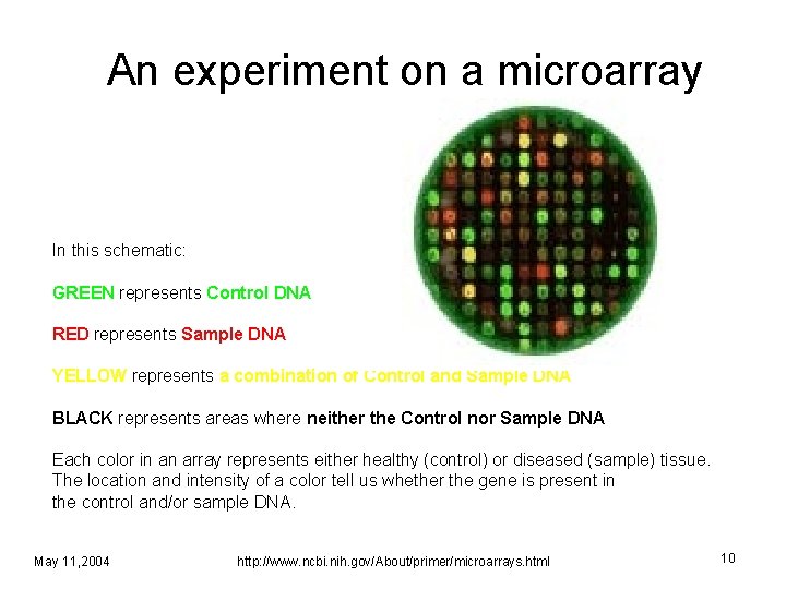
An experiment on a microarray In this schematic: GREEN represents Control DNA RED represents Sample DNA YELLOW represents a combination of Control and Sample DNA BLACK represents areas where neither the Control nor Sample DNA Each color in an array represents either healthy (control) or diseased (sample) tissue. The location and intensity of a color tell us whether the gene is present in the control and/or sample DNA. May 11, 2004 http: //www. ncbi. nih. gov/About/primer/microarrays. html 10

An Introduction to Bioinformatics Algorithms www. bioalgorithms. info DNA Microarray Millions of DNA strands build up on each location. 11/3/2020 May, 11, 2004 Tagged probes become hybridized to the DNA chip’s microarray. http: //www. affymetrix. com/corporate/media/image_library_1. affx 5

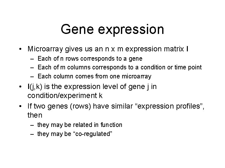
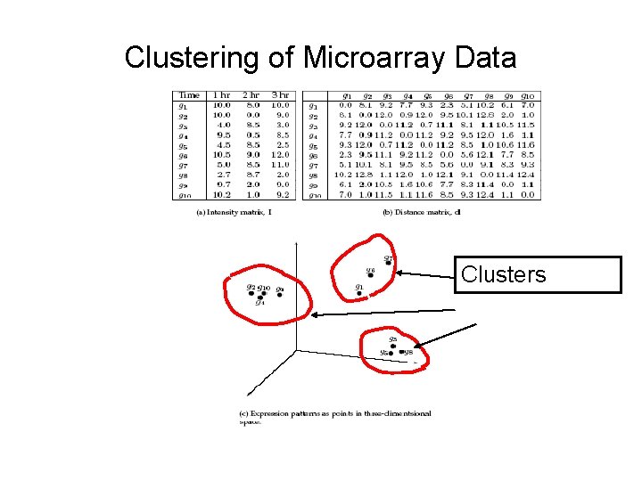
Gene expression • Microarray gives us an n x m expression matrix I – Each of n rows corresponds to a gene – Each of m columns corresponds to a condition or time point – Each column comes from one microarray • I(j, k) is the expression level of gene j in condition/experiment k • If two genes (rows) have similar “expression profiles”, then – they may be related in function – they may be “co-regulated”

Clustering • Find groups of genes that have similar expression profiles to one another • Such groups may be functionally related, and/or co-regulated • Compute pairwise distance metric d(i, j) for every pair of genes i and j • This gives an n x n “distance matrix” d

Goal of clustering • To group together genes into clusters such that – Genes within a cluster have highly similar expression profiles (small d(i, j)): “homogeneity” – Genes in different clusters have very different expression profiles (large d(i, j)): “separation” • “Good” clustering is one that adheres to these goals • A really “good” clustering is decided by biological interpretation of the clusters

Clustering of Microarray Data Clusters

Clustering problems • How to measure distance/similarity ? • How many clusters ? • Very large data sets: ~10, 000 gene, ~100 conditions create computational difficulties

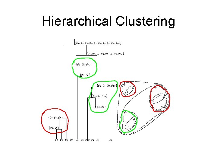
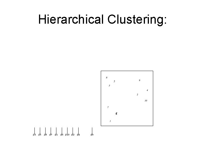
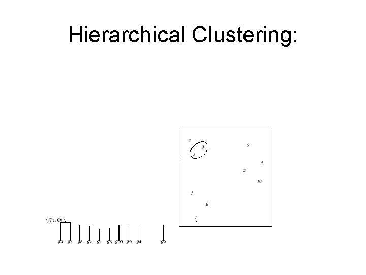
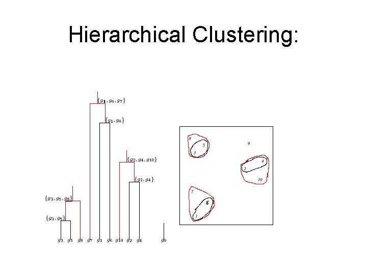
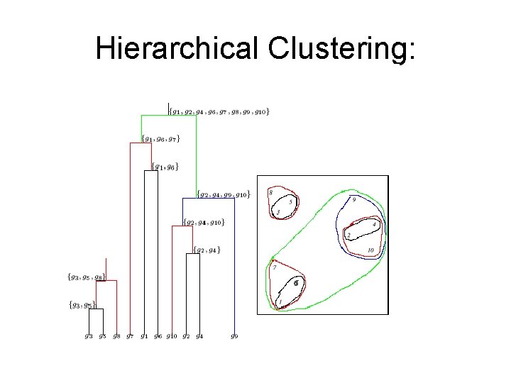
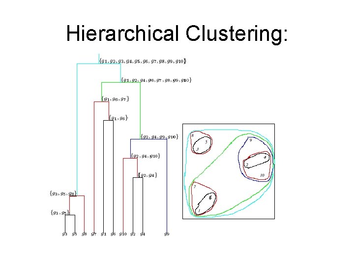
Hierarchical clustering • One approach to clustering • Does not explicitly partition genes into groups • Organizes genes into a tree; genes are at the leaves of the tree • Edges have lengths • Total path length between two genes (leaves) correlates with the distance between the genes

Hierarchical Clustering

Hierarchical Clustering: Example

Hierarchical Clustering: Example

Hierarchical Clustering: Example

Hierarchical Clustering: Example

Hierarchical Clustering: Example

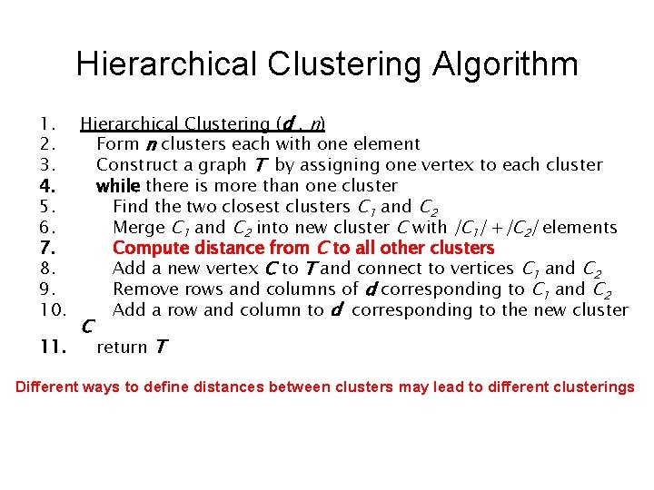
Hierarchical Clustering Algorithm 1. Hierarchical Clustering (d , n) 2. Form n clusters each with one element 3. Construct a graph T by assigning one vertex to each cluster 4. while there is more than one cluster 5. Find the two closest clusters C 1 and C 2 6. Merge C 1 and C 2 into new cluster C with |C 1| +|C 2| elements 7. Compute distance from C to all other clusters 8. Add a new vertex C to T and connect to vertices C 1 and C 2 9. Remove rows and columns of d corresponding to C 1 and C 2 10. Add a row and column to d corresponding to the new cluster C 11. return T Different ways to define distances between clusters may lead to different clusterings

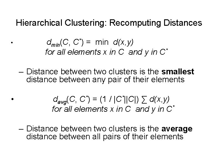
Hierarchical Clustering: Recomputing Distances • dmin(C, C*) = min d(x, y) for all elements x in C and y in C* – Distance between two clusters is the smallest distance between any pair of their elements • davg(C, C*) = (1 / |C*||C|) ∑ d(x, y) for all elements x in C and y in C* – Distance between two clusters is the average distance between all pairs of their elements

K-means clustering • Another popular solution to the clustering problem • Guess a number k, which is the number of clusters that will be reported • Finds explicit clusters (unlike hierarchical clustering)

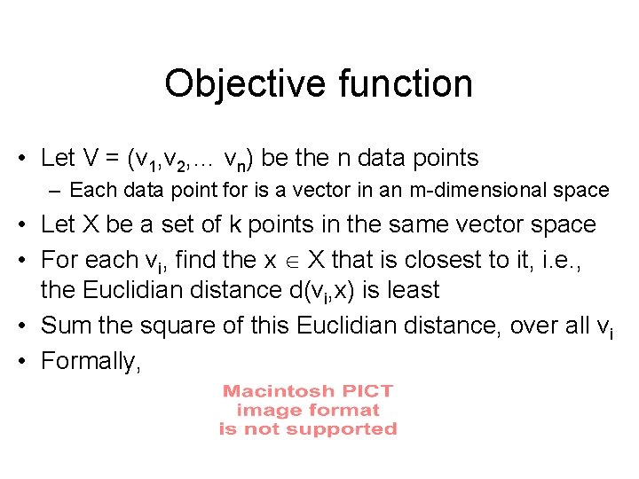
Objective function • Let V = (v 1, v 2, … vn) be the n data points – Each data point for is a vector in an m-dimensional space • Let X be a set of k points in the same vector space • For each vi, find the x X that is closest to it, i. e. , the Euclidian distance d(vi, x) is least • Sum the square of this Euclidian distance, over all vi • Formally,

Objective function • Find X such that d(V, X) is minimized • Input: A set, V, consisting of n points and a parameter k • Output: A set X consisting of k points (cluster centers) that minimizes the d(V, X) over all possible choices of X • An NP-complete problem for k > 1 • Easy for k=1 !

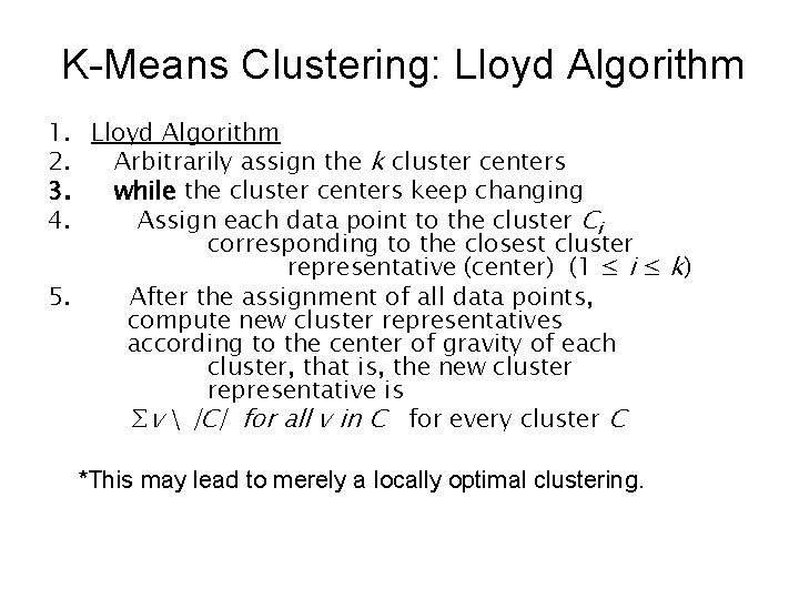
K-Means Clustering: Lloyd Algorithm 1. Lloyd Algorithm 2. Arbitrarily assign the k cluster centers 3. while the cluster centers keep changing 4. Assign each data point to the cluster Ci corresponding to the closest cluster representative (center) (1 ≤ i ≤ k) 5. After the assignment of all data points, compute new cluster representatives according to the center of gravity of each cluster, that is, the new cluster representative is ∑v |C| for all v in C for every cluster C *This may lead to merely a locally optimal clustering.

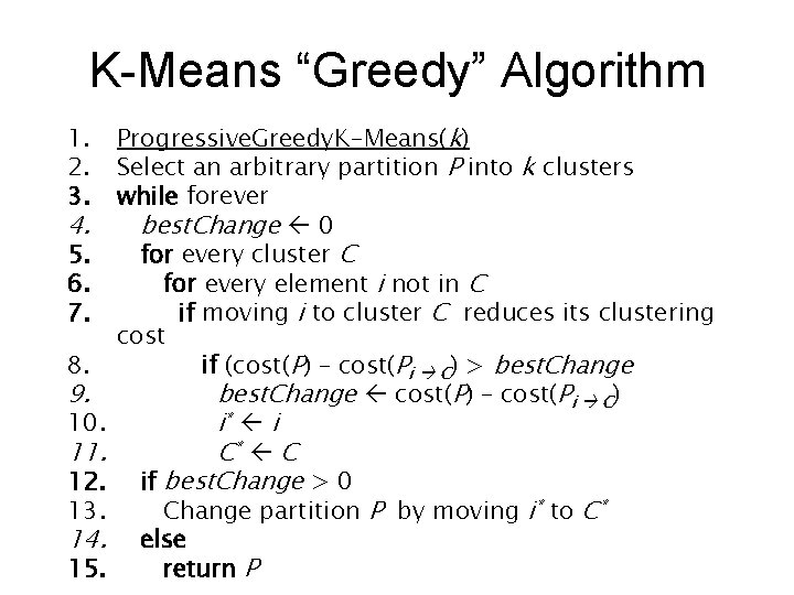
Conservative K-Means Algorithm • Lloyd algorithm is fast but in each iteration it moves many data points, not necessarily causing better convergence. A more conservative method would be to move one point at a time only if it improves the overall clustering cost • • • The smaller the clustering cost of a partition of data points is, the better that clustering is Different methods (e. g. , d(V, X) we saw earlier) can be used to measure this clustering cost

K-Means “Greedy” Algorithm 1. 2. 3. 4. 5. 6. 7. 8. 9. 10. 11. 12. 13. 14. 15. Progressive. Greedy. K-Means(k) Select an arbitrary partition P into k clusters while forever best. Change 0 for every cluster C for every element i not in C if moving i to cluster C reduces its clustering cost if (cost(P) – cost(Pi C) > best. Change cost(P) – cost(Pi C) i* i C* C if best. Change > 0 Change partition P by moving i* to C* else return P

Corrupted Cliques problem • Another approach to clustering • Based on the concept of “cliques” • Uses threshold on pairwise distance to decide which genes are “close” and which genes are “distant” • Builds a graph with edge between every pair of “close” genes

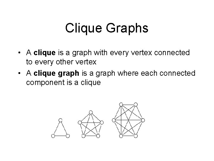
Clique Graphs • A clique is a graph with every vertex connected to every other vertex • A clique graph is a graph where each connected component is a clique

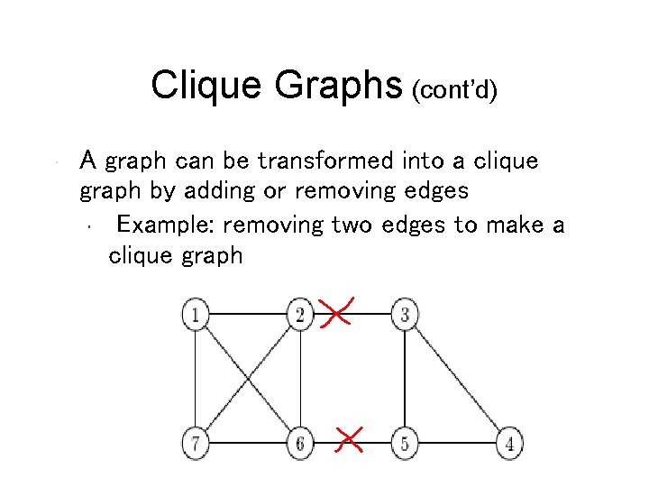
Clique Graphs (cont’d) • A graph can be transformed into a clique graph by adding or removing edges • Example: removing two edges to make a clique graph

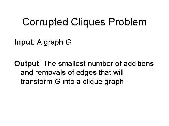
Corrupted Cliques Problem Input: A graph G Output: The smallest number of additions and removals of edges that will transform G into a clique graph

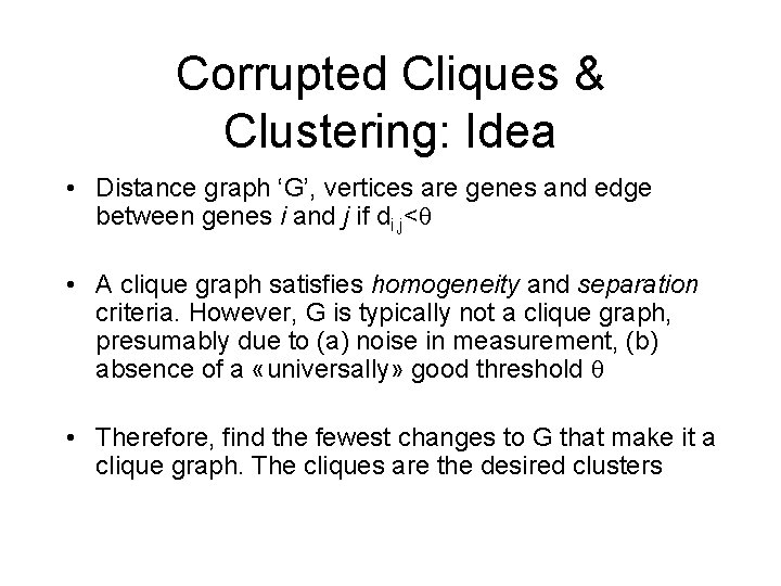
Corrupted Cliques & Clustering: Idea • Distance graph ‘G’, vertices are genes and edge between genes i and j if di, j< • A clique graph satisfies homogeneity and separation criteria. However, G is typically not a clique graph, presumably due to (a) noise in measurement, (b) absence of a «universally» good threshold • Therefore, find the fewest changes to G that make it a clique graph. The cliques are the desired clusters

Heuristics for Corrupted Clique Problem • Corrupted Cliques problem is NP-Hard, some heuristics exist to approximately solve it: • PCC (Parallel classification with cores): a time consuming algorithm • CAST (Cluster Affinity Search Technique): a practical and fast algorithm.

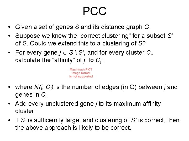
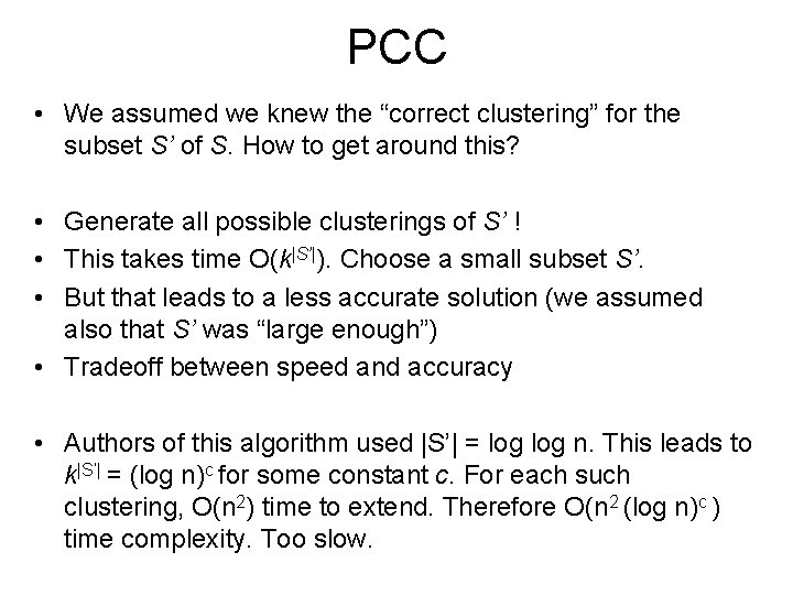
PCC • Given a set of genes S and its distance graph G. • Suppose we knew the “correct clustering” for a subset S’ of S. Could we extend this to a clustering of S? • For every gene j S S’, and for every cluster Ci, calculate the “affinity” of j to Ci : • where N(j, Ci) is the number of edges (in G) between j and genes in Ci. • Add every unclustered gene j to its maximum affinity cluster • If S’ is sufficiently large, and clustering of S’ is correct, then the above approach is likely to be correct.

PCC • We assumed we knew the “correct clustering” for the subset S’ of S. How to get around this? • Generate all possible clusterings of S’ ! • This takes time O(k|S’|). Choose a small subset S’. • But that leads to a less accurate solution (we assumed also that S’ was “large enough”) • Tradeoff between speed and accuracy • Authors of this algorithm used |S’| = log n. This leads to k|S’| = (log n)c for some constant c. For each such clustering, O(n 2) time to extend. Therefore O(n 2 (log n)c ) time complexity. Too slow.

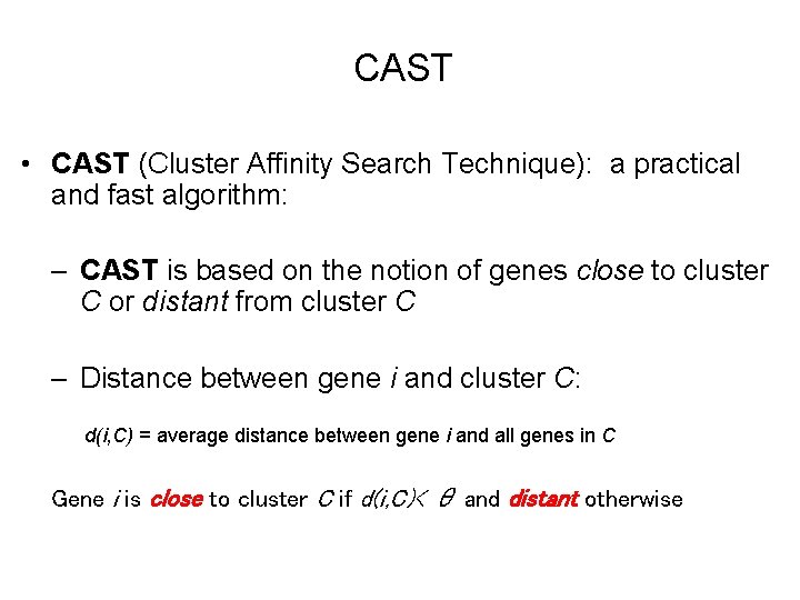
CAST • CAST (Cluster Affinity Search Technique): a practical and fast algorithm: – CAST is based on the notion of genes close to cluster C or distant from cluster C – Distance between gene i and cluster C: d(i, C) = average distance between gene i and all genes in C Gene i is close to cluster C if d(i, C)< θ and distant otherwise

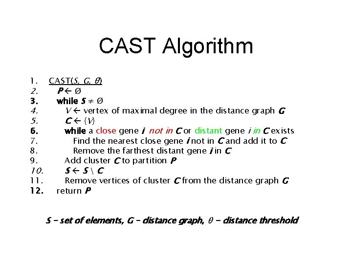
CAST Algorithm CAST(S, G, θ) 2. P Ø 3. while S ≠ Ø 4. V vertex of maximal degree in the distance graph G 5. C {V } 6. while a close gene i not in C or distant gene i in C exists 7. Find the nearest close gene i not in C and add it to C 8. Remove the farthest distant gene i in C 9. Add cluster C to partition P 10. S SC 11. Remove vertices of cluster C from the distance graph G 12. return P 1. S – set of elements, G – distance graph, θ - distance threshold