Gene Discovery The Central Dogma Transcription RNA polymerase

Gene Discovery

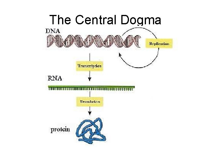
The Central Dogma

Transcription • RNA polymerase is the enzyme that builds an RNA strand from a gene • RNA that is transcribed from a gene is called messenger RNA (m. RNA)

RNA • RNA is like DNA except: – backbone is a little different – usually single stranded – the base uracil (U) is used in place of thymine (T) • A strand of RNA can be thought of as a string composed of the four letters: A, C, G, U

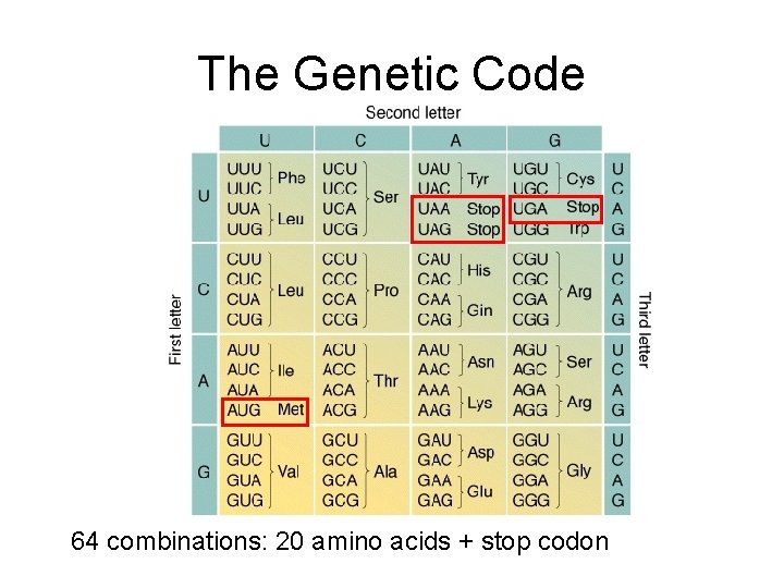
The Genetic Code 64 combinations: 20 amino acids + stop codon

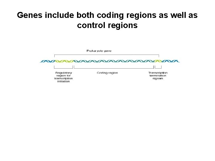
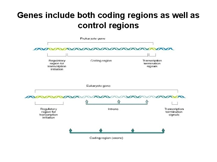
Genes include both coding regions as well as control regions

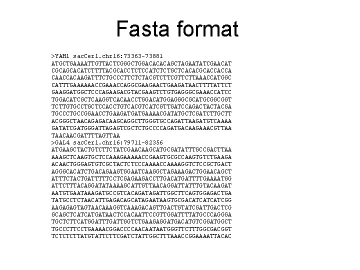
Fasta format >YAH 1 sac. Cer 1. chr 16: 73363 -73881 ATGCTGAAAATTGTTACTCGGGCTGGACACACAGCTAGAATATCGAACAT CGCAGCACATCTTTTACGCACCTCTCCATCTCTGCTCACACGCACCACCA CAACCACAAGATTTCTGCCCTTCTCTACGTCTTCGTTCTTAAACCATGGC CATTTGAAAAAACCGAAACCAGGCGAAGAACTGAAGATAACTTTTATTCT GAAGGATGGCTCCCAGAAGACGTACGAAGTCTGTGAGGGCGAAACCATCC TGGACATCGCTCAAGGTCACAACCTGGACATGGAGGGCGCATGCGGCGGT TCTTGTGCCTGCTCCACCTGTCACGTCATCGTTGATCCAGACTACTACGA TGCCCTGCCGGAACCTGAAGATGATGAAAACGATATGCTCGATCTTGCTT ACGGGCTAACAGAGACAAGCAGGCTTGGGTGCCAGATTAAGATGTCAAAA GATATCGATGGGATTAGAGTCGCTCTGCCCCAGATGACAAGAAACGTTAA TAACAACGATTTTAGTTAA >GAL 4 sac. Cer 1. chr 16: 79711 -82356 ATGAAGCTACTGTCTTCTATCGAACAAGCATGCGATATTTGCCGACTTAA AAAGCTCAAGTGCTCCAAAGAAAAACCGAAGTGCGCCAAGTGTCTGAAGA ACAACTGGGAGTGTCGCTACTCTCCCAAAAGGTCTCCGCTGACT AGGGCACATCTGACAGAAGTGGAATCAAGGCTAGAAAGACTGGAACAGCT ATTTCTACTGATTTTTCCTCGAGAAGACCTTGACATGATTTTGAAAATGG ATTCTTTACAGGATATAAAAGCATTGTTAACAGGATTATTTGTACAAGAT AATGTGAATAAAGATGCCGTCACAGATTGGCTTCAGTGGAGACTGA TATGCCTCTAACATTGAGACAGCATAGAATAAGTGCGACATCATCATCGG AAGAGAGTAGTAACAAAGGTCAAAGACAGTTGACTGTATCGATTGACTCG GCAGCTCATCATGATAACTCCACAATTCCGTTGGATTTTATGCCCAGGGA TGCTCTTCATGGATTTGATTGGTCTGAAGAGGATGACATGTCGGATGGCT TGCCCTTCCTGAAAACGGACCCCAACAATAATGGGTTCTTTGGCGACGGT TCTCTCTTATGTATTCTTCGATCTATTGGCTTTAAACCGGAAAATTACAC

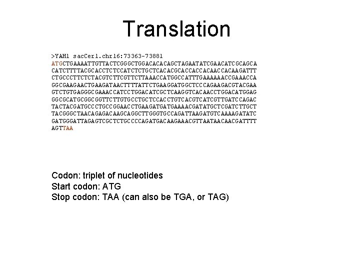
Translation >YAH 1 sac. Cer 1. chr 16: 73363 -73881 ATGCTGAAAATTGTTACTCGGGCTGGACACACAGCTAGAATATCGAACATCGCAGCA CATCTTTTACGCACCTCTCCATCTCTGCTCACACGCACCACCACAAGATTT CTGCCCTTCTCTACGTCTTCGTTCTTAAACCATGGCCATTTGAAAAAACCGAAACCA GGCGAAGAACTGAAGATAACTTTTATTCTGAAGGATGGCTCCCAGAAGACGTACGAA GTCTGTGAGGGCGAAACCATCCTGGACATCGCTCAAGGTCACAACCTGGACATGGAG GGCGCATGCGGCGGTTCTTGTGCCTGCTCCACCTGTCACGTCATCGTTGATCCAGAC TACTACGATGCCCTGCCGGAACCTGAAGATGATGAAAACGATATGCTCGATCTTGCT TACGGGCTAACAGAGACAAGCAGGCTTGGGTGCCAGATTAAGATGTCAAAAGATATC GATGGGATTAGAGTCGCTCTGCCCCAGATGACAAGAAACGTTAATAACAACGATTTT AGTTAA Codon: triplet of nucleotides Start codon: ATG Stop codon: TAA (can also be TGA, or TAG)

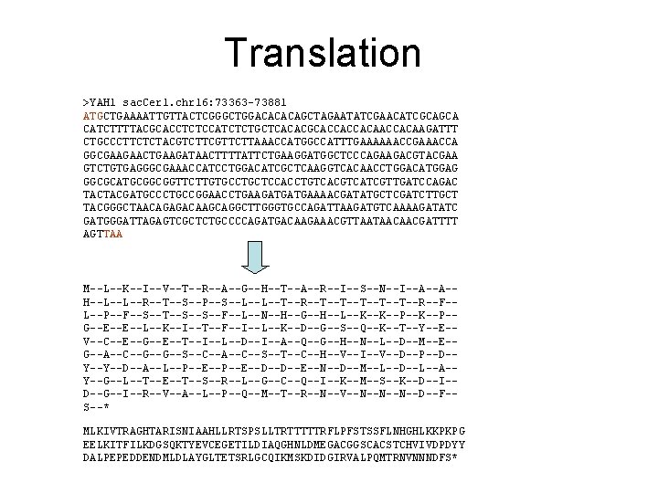
Translation >YAH 1 sac. Cer 1. chr 16: 73363 -73881 ATGCTGAAAATTGTTACTCGGGCTGGACACACAGCTAGAATATCGAACATCGCAGCA CATCTTTTACGCACCTCTCCATCTCTGCTCACACGCACCACCACAAGATTT CTGCCCTTCTCTACGTCTTCGTTCTTAAACCATGGCCATTTGAAAAAACCGAAACCA GGCGAAGAACTGAAGATAACTTTTATTCTGAAGGATGGCTCCCAGAAGACGTACGAA GTCTGTGAGGGCGAAACCATCCTGGACATCGCTCAAGGTCACAACCTGGACATGGAG GGCGCATGCGGCGGTTCTTGTGCCTGCTCCACCTGTCACGTCATCGTTGATCCAGAC TACTACGATGCCCTGCCGGAACCTGAAGATGATGAAAACGATATGCTCGATCTTGCT TACGGGCTAACAGAGACAAGCAGGCTTGGGTGCCAGATTAAGATGTCAAAAGATATC GATGGGATTAGAGTCGCTCTGCCCCAGATGACAAGAAACGTTAATAACAACGATTTT AGTTAA M--L--K--I--V--T--R--A--G--H--T--A--R--I--S--N--I--A--A-H--L--L--R--T--S--P--S--L--L--T--R--T--T--T--R--F-L--P--F--S--T--S--S--F--L--N--H--G--H--L--K--K--P-G--E--E--L--K--I--T--F--I--L--K--D--G--S--Q--K--T--Y--E-V--C--E--G--E--T--I--L--D--I--A--Q--G--H--N--L--D--M--E-G--A--C--G--G--S--C--A--C--S--T--C--H--V--I--V--D--P--D-Y--Y--D--A--L--P--E--D--D--E--N--D--M--L--D--L--A-Y--G--L--T--E--T--S--R--L--G--C--Q--I--K--M--S--K--D--I-D--G--I--R--V--A--L--P--Q--M--T--R--N--V--N--N--N--D--F-S--* MLKIVTRAGHTARISNIAAHLLRTSPSLLTRTTTTTRFLPFSTSSFLNHGHLKKPKPG EELKITFILKDGSQKTYEVCEGETILDIAQGHNLDMEGACGGSCACSTCHVIVDPDYY DALPEPEDDENDMLDLAYGLTETSRLGCQIKMSKDIDGIRVALPQMTRNVNNNDFS*

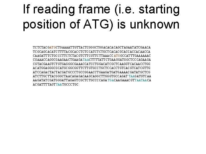
If reading frame (i. e. starting position of ATG) is unknown TCTCTACGATGCTGAAAATTGTTACTCGGGCTGGACACACAGCTAGAATATCGAACA TCGCAGCACATCTTTTACGCACCTCTCCATCTCTGCTCACACGCACCACCACAACCA CAAGATTTCTGCCCTTCTCTACGTCTTCGTTCTTAAACC ATGGCCATTTGAAAAAAC CGAAACCAGGCGAAGAACTGAAGA TAACTTTTATTCTGAAGGATGGCTCCCAGAAGA CGTACGAAGTCTGTGAGGGCGAAACCATCCTGGACATCGCTCAAGGTCACAACCTGG ACATGGAGGGCGCATGCGGCGGTTCTTGTGCCTGCTCCACCTGTCACGTCATCGTTG ATCCAGACTACTACGATGCCCTGCCGGAACCTGAAGATGATGAAAACGATATGCTCG ATCTTGCTTACGGGCTAACAGAGACAAGCAGGCTTGGGTGCCAGAT TAAGATGTCAA AAGATATCGATGGGATTAGAGTCGCTCTGCCCCAGA TGACAAGAAACGTTAATAACA ACGATTTTAGTTAATGCCCTGC

Open reading frame (ORF) • One can represent a genome of length n as a sequence of n/3 codons • The three ‘stop’ codons (TAA, TAG, and TGA) break this sequence into segments, one between every two consecutive stop codons • The subsegments of these that start from a start codon (ATG) are ORFs

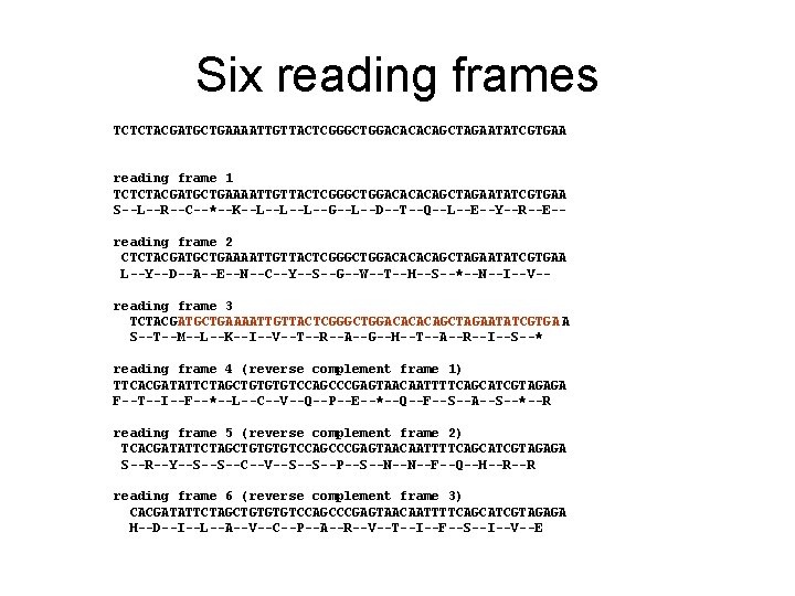
Six reading frames TCTCTACGATGCTGAAAATTGTTACTCGGGCTGGACACACAGCTAGAATATCGTGAA reading frame 1 TCTCTACGATGCTGAAAATTGTTACTCGGGCTGGACACACAGCTAGAATATCGTGAA S--L--R--C--*--K--L--L--L--G--L--D--T--Q--L--E--Y--R--E-reading frame 2 CTCTACGATGCTGAAAATTGTTACTCGGGCTGGACACACAGCTAGAATATCGTGAA L--Y--D--A--E--N--C--Y--S--G--W--T--H--S--*--N--I--V-reading frame 3 TCTACGATGCTGAAAATTGTTACTCGGGCTGGACACACAGCTAGAATATCGTGA A S--T--M--L--K--I--V--T--R--A--G--H--T--A--R--I--S--* reading frame 4 (reverse complement frame 1) TTCACGATATTCTAGCTGTGTGTCCAGCCCGAGTAACAATTTTCAGCATCGTAGAGA F--T--I--F--*--L--C--V--Q--P--E--*--Q--F--S--A--S--*--R reading frame 5 (reverse complement frame 2) TCACGATATTCTAGCTGTGTGTCCAGCCCGAGTAACAATTTTCAGCATCGTAGAGA S--R--Y--S--S--C--V--S--S--P--S--N--N--F--Q--H--R--R reading frame 6 (reverse complement frame 3) CACGATATTCTAGCTGTGTGTCCAGCCCGAGTAACAATTTTCAGCATCGTAGAGA H--D--I--L--A--V--C--P--A--R--V--T--I--F--S--I--V--E

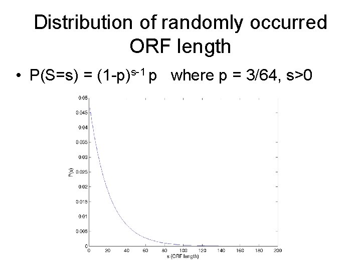
Size of ORF • Total number of codons: 43 = 64 • Assuming random occurrences of A, C, G, Ts with equal probability: • The probability of a codon being start codon is: 1/64 • The probability of a codon being stop codon is: 3/64 Define S to be the length of an ORF (the number of codons, excluding the stop-codon) If sequences are randomly generated (A, C, G, T with equal chance), then S is a random variable. Question: what is the probability distribution of S ?

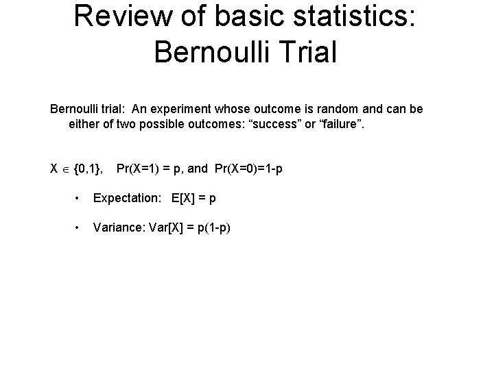
Review of basic statistics: Bernoulli Trial Bernoulli trial: An experiment whose outcome is random and can be either of two possible outcomes: “success” or “failure”. X {0, 1}, Pr(X=1) = p, and Pr(X=0)=1 -p • Expectation: E[X] = p • Variance: Var[X] = p(1 -p)

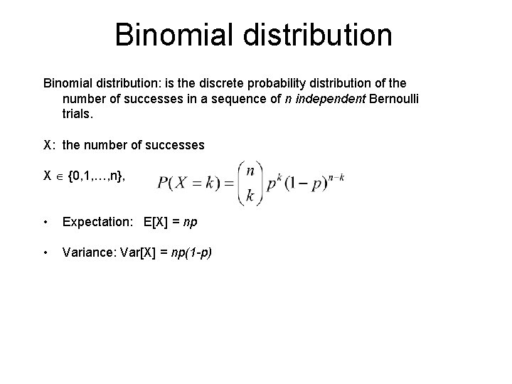
Binomial distribution: is the discrete probability distribution of the number of successes in a sequence of n independent Bernoulli trials. X: the number of successes X {0, 1, …, n}, • Expectation: E[X] = np • Variance: Var[X] = np(1 -p)

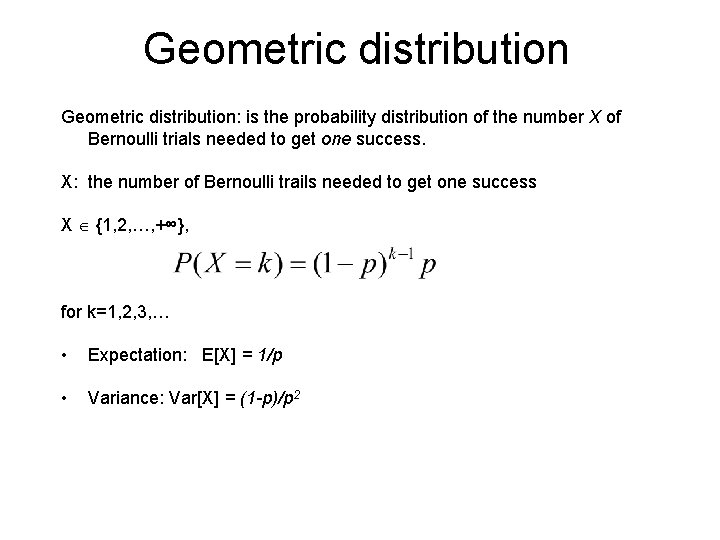
Geometric distribution: is the probability distribution of the number X of Bernoulli trials needed to get one success. X: the number of Bernoulli trails needed to get one success X {1, 2, …, +∞}, for k=1, 2, 3, … • Expectation: E[X] = 1/p • Variance: Var[X] = (1 -p)/p 2

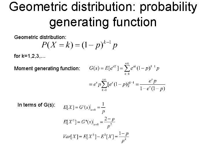
Geometric distribution: probability generating function Geometric distribution: for k=1, 2, 3, … Moment generating function: In terms of G(s):

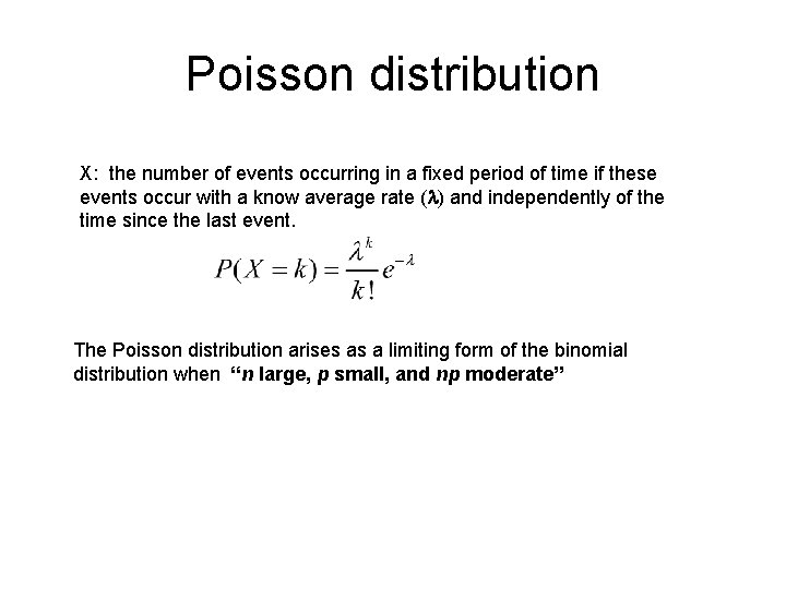
Poisson distribution X: the number of events occurring in a fixed period of time if these events occur with a know average rate ( ) and independently of the time since the last event. The Poisson distribution arises as a limiting form of the binomial distribution when “n large, p small, and np moderate”

Distribution of randomly occurred ORF length • P(S=s) = (1 -p)s-1 p where p = 3/64, s>0

Statistical hypothesis testing A statistical hypothesis test is a method of making statistical decisions using experimental data. A result is called statistically significant if it is unlikely to have occurred by chance. These decisions are almost always made using null-hypothesis tests, that is, ones that answer the question: “Assuming that the null hypothesis is true, what is the probability of observing a value for the test statistic that is at least as extreme as the value that was actually observed?

Coin flipping example A coin flipping experiment: Flip a coin 10 times. Suppose the outcome is {1 1 0 1 1 1}, that is, 8 heads and 2 tails. Null hypothesis: H 0: This is a normal, unbiased coin (i. e. has equal probabilities of producing a head or a tail. Test static: T=8 (number of heads observed)

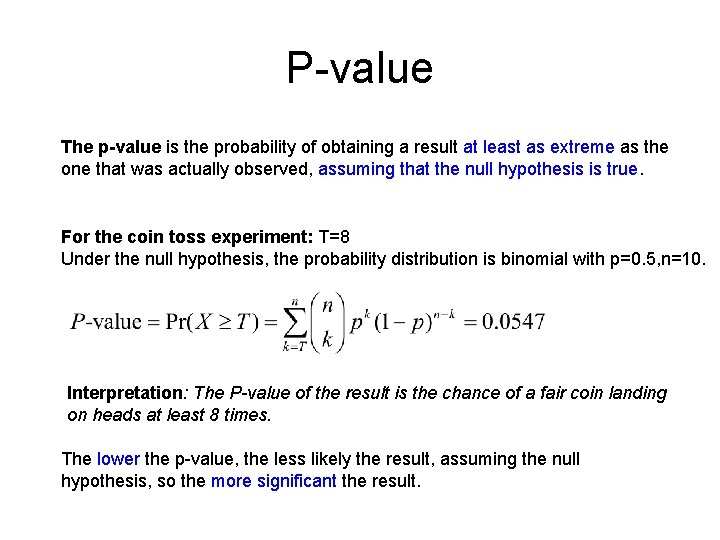
P-value The p-value is the probability of obtaining a result at least as extreme as the one that was actually observed, assuming that the null hypothesis is true. For the coin toss experiment: T=8 Under the null hypothesis, the probability distribution is binomial with p=0. 5, n=10. Interpretation: The P-value of the result is the chance of a fair coin landing on heads at least 8 times. The lower the p-value, the less likely the result, assuming the null hypothesis, so the more significant the result.

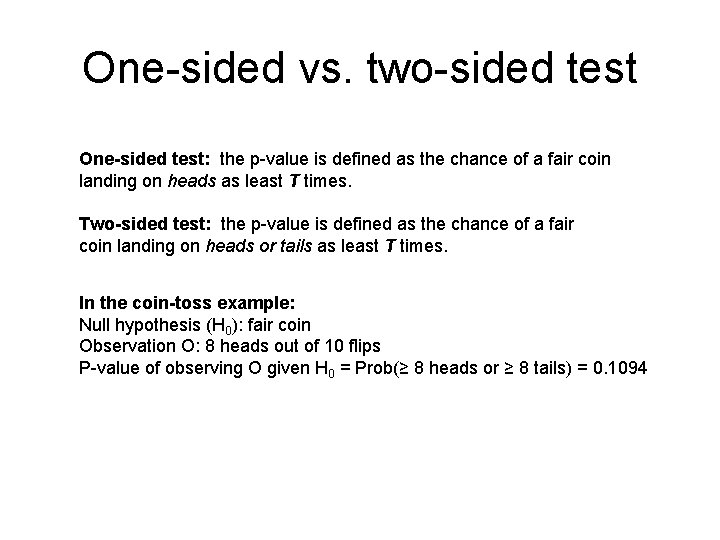
One-sided vs. two-sided test One-sided test: the p-value is defined as the chance of a fair coin landing on heads as least T times. Two-sided test: the p-value is defined as the chance of a fair coin landing on heads or tails as least T times. In the coin-toss example: Null hypothesis (H 0): fair coin Observation O: 8 heads out of 10 flips P-value of observing O given H 0 = Prob(≥ 8 heads or ≥ 8 tails) = 0. 1094

Null hypothesis test A null hypothesis is never proven by such methods, as the absence of evidence against the null hypothesis does not establish its truth. In other words, one may either reject, or not reject the null hypothesis; one cannot accept it. This means that one cannot make decisions or draw conclusions that assume the truth of the null hypothesis.

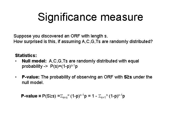
Significance measure Suppose you discovered an ORF with length s. How surprised is this, if assuming A, C, G, Ts are randomly distributed? Statistics: • Null model: A, C, G, Ts are randomly distributed with equal probability -> P(s)=(1 -p)s-1 p • P-value: The probability of observing an ORF with S≥s under the null model. P-value = P(S≥s) = x=s (1 -p)x-1 p = 1 - x=1 s (1 -p)x-1 p

Student’s t-test A t-test is any statistical hypothesis test in which the test statistic follows a Student’s t distribution if the null hypothesis is true.

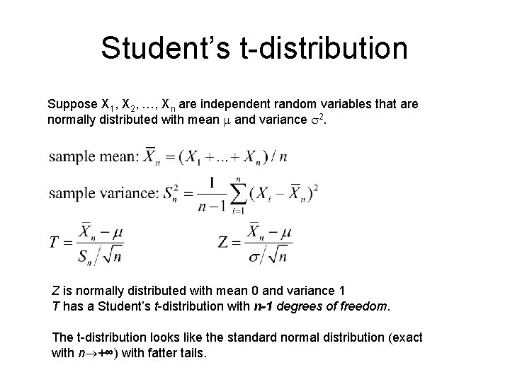
Student’s t-distribution Suppose X 1, X 2, …, Xn are independent random variables that are normally distributed with mean m and variance s 2. Z is normally distributed with mean 0 and variance 1 T has a Student’s t-distribution with n-1 degrees of freedom. The t-distribution looks like the standard normal distribution (exact with n +∞) with fatter tails.

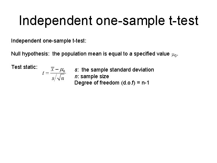
Independent one-sample t-test: Null hypothesis: the population mean is equal to a specified value m 0. Test static: s: the sample standard deviation n: sample size Degree of freedom (d. o. f) = n-1

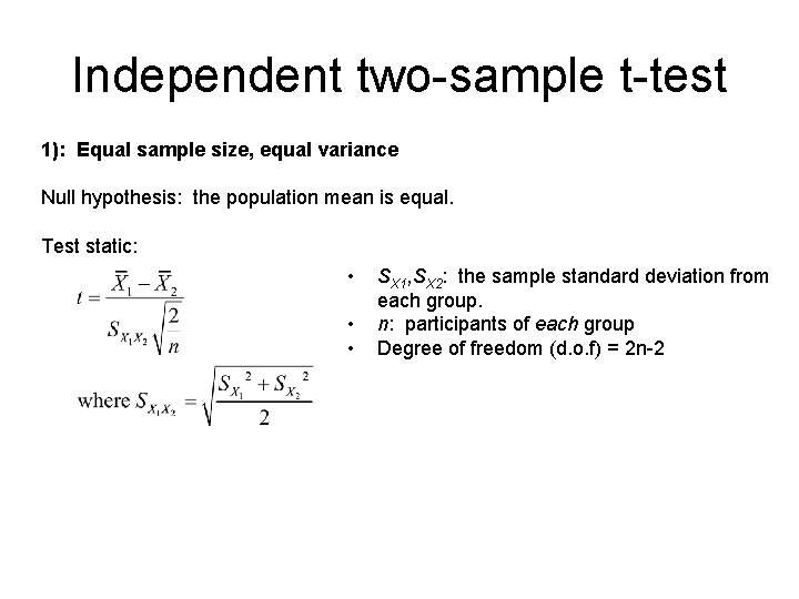
Independent two-sample t-test 1): Equal sample size, equal variance Null hypothesis: the population mean is equal. Test static: • • • SX 1, SX 2: the sample standard deviation from each group. n: participants of each group Degree of freedom (d. o. f) = 2 n-2

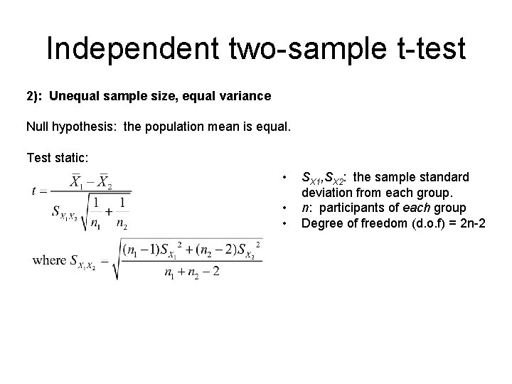
Independent two-sample t-test 2): Unequal sample size, equal variance Null hypothesis: the population mean is equal. Test static: • • • SX 1, SX 2: the sample standard deviation from each group. n: participants of each group Degree of freedom (d. o. f) = 2 n-2

Gene discovery in higher order organisms More complicated than ORF discovery due to more complex gene structure: multiple exons separated by introns. Methods: 1. Statistical models of codon usage 2. Markov models of gene structure 3. Comparing across different species

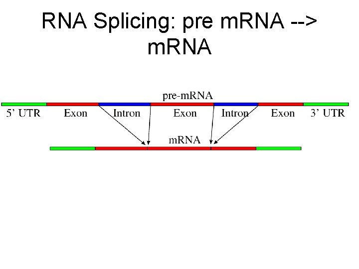
RNA Splicing: pre m. RNA --> m. RNA

Genes include both coding regions as well as control regions