Gene by environment effects Elevated Plus Maze anxiety

Gene by environment effects

")
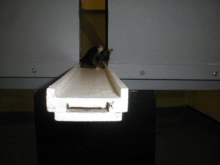
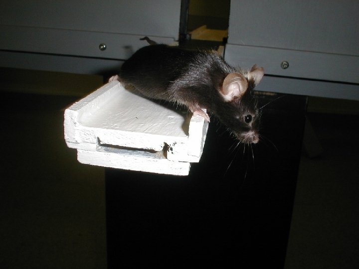
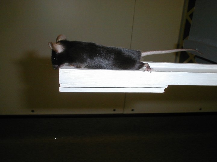
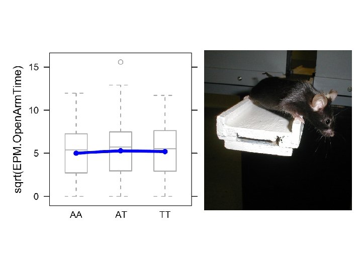
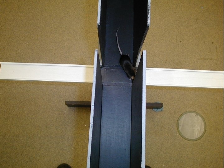
Elevated Plus Maze (anxiety)

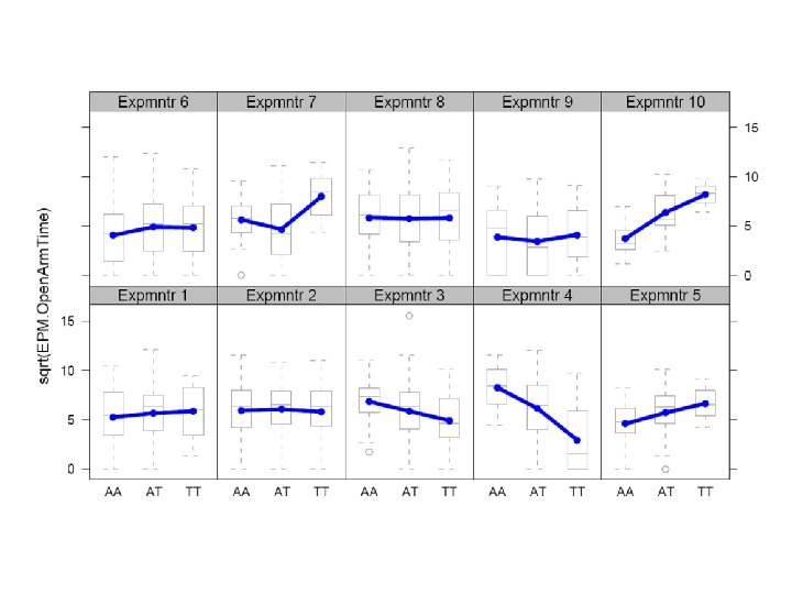

Modelling E, G and Gx. E H 0 : phenotype ~ 1 H 1 : phenotype ~ covariate H 2 : phenotype ~ covariate + Locus. X H 3 : phenotype ~ covariate + Locus. X + covariate: Locus. X

PRACTICAL: Inclusion of gender effects in a genome scan To start: 1. Copy the folder facultyvaldarFriday. Animal. Models. Practical to your own directory. 2. Start R 3. File -> Change Dir… and change directory to your Friday. Animal. Models. Practical directory 4. Open Firefox, then File -> Open File, and open “gxe. R” in the Friday. Animal. Models. Practical directory

H 0 : phenotype ~ sex H 1 : phenotype ~ sex + marker

H 0 : phenotype ~ sex H 1 : phenotype ~ sex + marker scan. markers(Phenotype ~ Sex + MARKER, h 0 = Phenotype ~ Sex, . . . etc)

H 0 : phenotype ~ sex H 1 : phenotype ~ sex + marker scan. markers(Phenotype ~ Sex + MARKER, h 0 = Phenotype ~ Sex, . . . etc)

H 0 : phenotype ~ sex H 1 : phenotype ~ sex + marker scan. markers(Phenotype ~ Sex + MARKER, h 0 = Phenotype ~ Sex, . . . etc)
 anova(lm(Phenotype ~ Sex + m 1 + Sex: m 1, data=ped.")
head(ped. gender 0) anova(lm(Phenotype ~ Sex + m 1 + Sex: m 1, data=ped. gender 0)) head(ped. gender 1) anova(lm(Phenotype ~ Sex + m 1 + Sex: m 1, data=ped. gender 1)

New approaches Advanced intercross lines Genetically heterogeneous stocks

F 2 Intercross x F 1 Avg. Distance Between Recombinations F 2 intercross ~30 c. M F 2
 F 0 F 1 F 2 F 3 F 4")
Advanced intercross lines (AILs) F 0 F 1 F 2 F 3 F 4
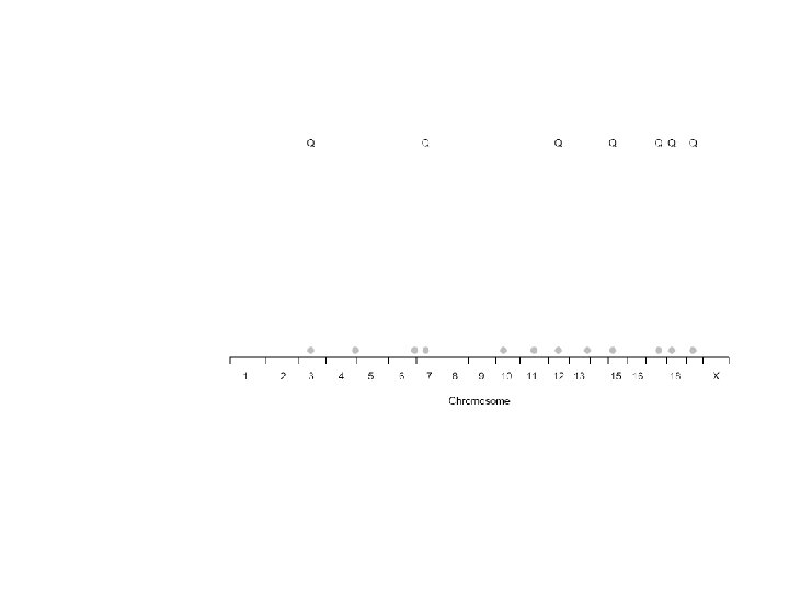
 significance threshold 0")
Chromosome scan for F 12 QTL goodness of fit (log. P) significance threshold 0 Typical chromosome position along whole chromosome (Mb) 100 c. M

PRACTICAL: AILs To start: 1. Open Firefox, then File -> Open File, and open “ail_and_ghosts. R” in the Friday. Animal. Models. Practical directory

Genetically Heterogeneous Mice

F 2 Intercross x F 1 Avg. Distance Between Recombinations F 2 intercross ~30 c. M F 2

Heterogeneous Stock F 2 Intercross x Pseudo-random mating for 50 generations F 1 Avg. Distance Between Recombinations: HS ~2 c. M F 2 intercross ~30 c. M F 2

Heterogeneous Stock F 2 Intercross x Pseudo-random mating for 50 generations F 1 Avg. Distance Between Recombinations: HS ~2 c. M F 2 intercross ~30 c. M F 2

Genome scans with single marker association

High resolution mapping

Relation Between Marker and Genetic Effect QTL Marker 1 Observable effect

Relation Between Marker and Genetic Effect Marker 2 QTL Marker 1 Observable effect

Relation Between Marker and Genetic Effect Marker 2 No effect observable QTL Marker 1 Observable effect
 calculates the probability that an allele descends from a founder using")
Multipoint method (HAPPY) calculates the probability that an allele descends from a founder using multiple markers Observed chromosome structure Hidden Chromosome Structure

Haplotype reconstruction using HAPPY chromosome genotypes haplotype proportions predicted by HAPPY

HAPPY model for additive effects

Genome scans with single marker association

Genome scans with HAPPY

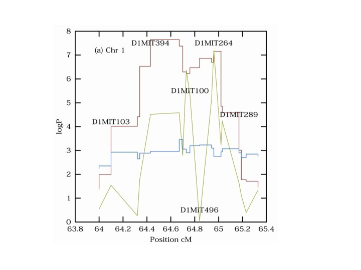
Results for our HS

Many peaks mean red cell volume


How to select peaks: a simulated example

How to select peaks: a simulated example Simulate 7 x 5% QTLs (ie, 35% genetic effect) + 20% shared environment effect + 45% noise = 100% variance

Simulated example: 1 D scan

Peaks from 1 D scan phenotype ~ covariates + ?

1 D scan: condition on 1 peak phenotype ~ covariates + peak 1 + ?

1 D scan: condition on 2 peaks phenotype ~ covariates + peak 1 + peak 2 + ?

1 D scan: condition on 3 peaks phenotype ~ covariates + peak 1 + peak 2 + peak 3 + ?

1 D scan: condition on 4 peaks phenotype ~ covariates + peak 1 + peak 2 + peak 3 + peak 4 + ?

1 D scan: condition on 5 peaks phenotype ~ covariates + peak 1 + peak 2 + peak 3 + peak 4 + peak 5 + ?

1 D scan: condition on 6 peaks phenotype ~ covariates + peak 1 + peak 2 + peak 3 + peak 4 + peak 5 + peak 6 + ?

1 D scan: condition on 7 peaks phenotype ~ covariates + peak 1 + peak 2 + peak 3 + peak 4 + peak 5 + peak 6 + peak 7 + ?

1 D scan: condition on 8 peaks phenotype ~ covariates + peak 1 + peak 2 + peak 3 + peak 4 + peak 5 + peak 6 + peak 7 + peak 8 + ?

1 D scan: condition on 9 peaks phenotype ~ covariates + peak 1 + peak 2 + peak 3 + peak 4 + peak 5 + peak 6 + peak 7 + peak 8 + peak 9 +?

1 D scan: condition on 10 peaks phenotype ~ covariates + peak 1 + peak 2 + peak 3 + peak 4 + peak 5 + peak 6 + peak 7 + peak 8 + peak 9 + peak 10 + ?

1 D scan: condition on 11 peaks phenotype ~ covariates + peak 1 + peak 2 + peak 3 + peak 4 + peak 5 + peak 6 + peak 7 + peak 8 + peak 9 + peak 10 + peak 11 + ?

Peaks chosen by forward selection

Bootstrap sampling 1 2 3 10 subjects 4 5 6 7 8 9 10

Bootstrap sampling sample with replacement 10 subjects 1 1 2 2 3 2 4 3 5 5 6 5 7 6 8 7 9 7 10 9 bootstrap sample from 10 subjects

Forward selection on a bootstrap sample

Forward selection on a bootstrap sample

Forward selection on a bootstrap sample

Bootstrap evidence mounts up…
")
In 1000 bootstraps… Bootstrap Posterior Probability (BPP)

Results

Tea Break

Study design 2, 000 mice 15, 000 diallelic markers More than 100 phenotypes each mouse subject to a battery of tests spread over weeks 5 -9 of the animal’s life
![101 Phenotypes Anxiety (conditioned and unconditioned tasks) [24] Asthma (plethysmography) [13] Biochemistry [15] Diabetes](http://slidetodoc.com/presentation_image_h/ab9d6a4000db2e4c209cff16bbf6a9d4/image-66.jpg "101 Phenotypes Anxiety (conditioned and unconditioned tasks) [24] Asthma (plethysmography) [13] Biochemistry [15] Diabetes")
101 Phenotypes Anxiety (conditioned and unconditioned tasks) [24] Asthma (plethysmography) [13] Biochemistry [15] Diabetes (glucose tolerance test) [16] Haematology [15] Immunology [9] Weight/size related [8] Wound Healing [1]

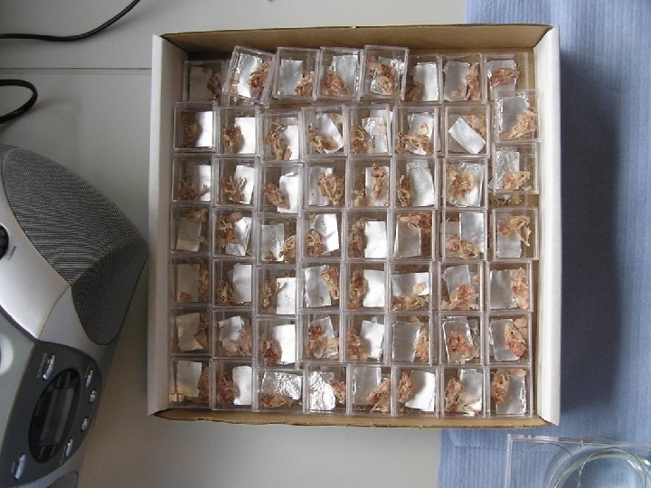
High throughput phenotyping facility

Photo ID

Open Field

Open Field Non anxious mouse Anxious mouse
")
Elevated Plus Maze (anxiety)


")
Food hyponeophagia (reluctance to try new food)

“Home Cage” activity

Startle & Conditioning

Plethysmograph

Plethysmograph
")
Glucose Tolerance Test (diabetes)

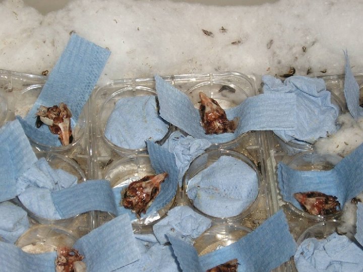
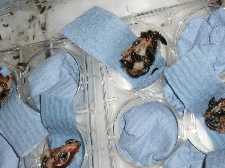
Wound healing

PRACTICAL: http: //gscan. well. ox. ac. uk

END

An individual’s phenotype follows a mixture of normal distributions

Paternal chromosome Maternal chromosome m

m Chromosome 1 Chromosome 2 Strains A B C D E F

Markers m Strains A B C D E F

Markers m Strains A B C D E F

Markers m 0. 5 c. M

Markers m 0. 5 c. M 1 c. M

Markers 0. 5 c. M 1 c. M m
: implemented in HAPPY http: //www. well. ox.")
Analysis Probabilistic Ancestral Haplotype Reconstruction (descent mapping): implemented in HAPPY http: //www. well. ox. ac. uk/~rmott/happy. html

M 1 m 1 Q q M 2 m 2 M 1 recombination ? m 2

m 1 M 1 M 1 m 1 Q q q Q q M 2 m 2

m 1 M 1 M 1 m 1 Q q q Q q M 2 m 2 M 1 m 1 M 1 Q q Q m 2 M 2 m 2

M 1 m 1 M 1 Q q q m 2 m 2 m 1 M 1 Q q Q M 2 m 2 m 1 Q q M 2 m 2

M 1 m 1 ? ? m 2 c. M distances determine probabilities

M 1 Eg, m 1 ? ? m 2 c. M distances determine probabilities

Interval mapping M 1 M 2 m 1 m 2 LOD score M 1 m 1 M 2 m 2

Interval mapping M 1 m 1 Q q M 2 m 2 LOD score M 1 m 1 M 2 m 2

Interval mapping M 1 m 1 Q q M 2 m 2 LOD score M 1 m 1 M 2 m 2

Interval mapping M 1 m 1 Q q M 2 m 2 LOD score M 1 m 1 M 2 m 2
- Slides: 107