Gaussian Mixture Model and the EM algorithm in

Gaussian Mixture Model and the EM algorithm in Speech Recognition Puskás János-Pál

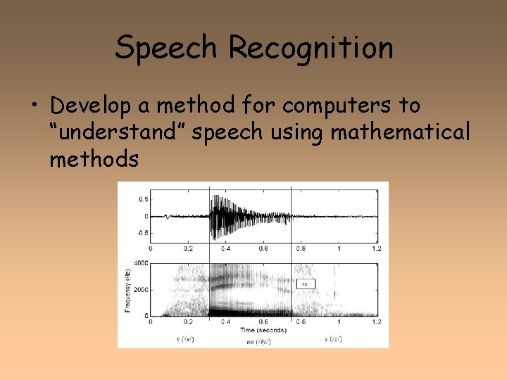
Speech Recognition • Develop a method for computers to “understand” speech using mathematical methods

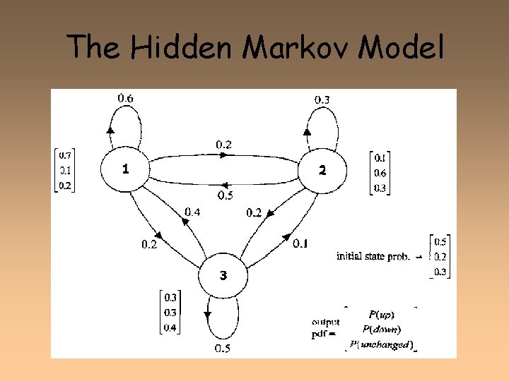
The Hidden Markov Model

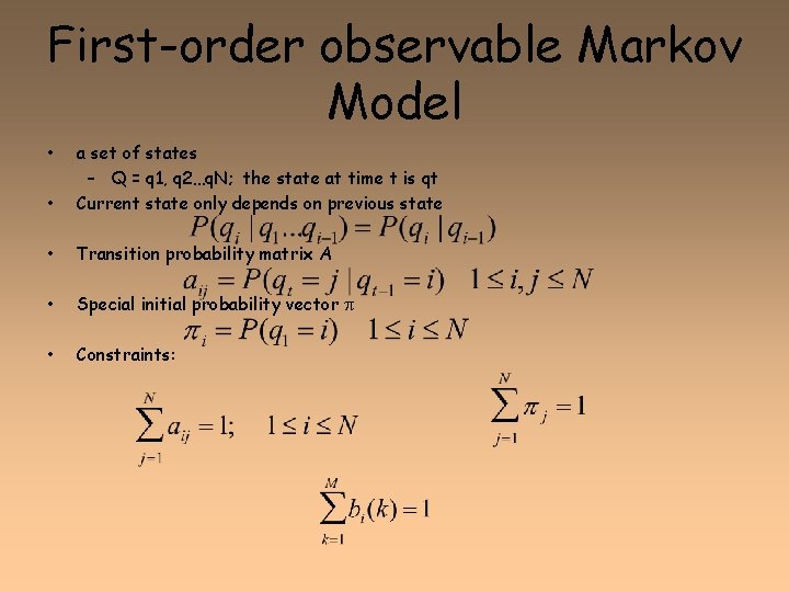
First-order observable Markov Model • • a set of states – Q = q 1, q 2…q. N; the state at time t is qt Current state only depends on previous state • Transition probability matrix A • Special initial probability vector • Constraints:

Problem: how to apply HMM model to continuous observations? • We have assumed that the output alphabet V has a finite number of symbols • But spectral feature vectors are realvalued! • How to deal with real-valued features? – Decoding: Given ot, how to compute P(ot|q) – Learning: How to modify EM to deal with real-valued features

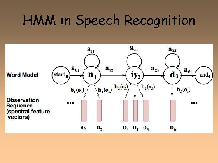
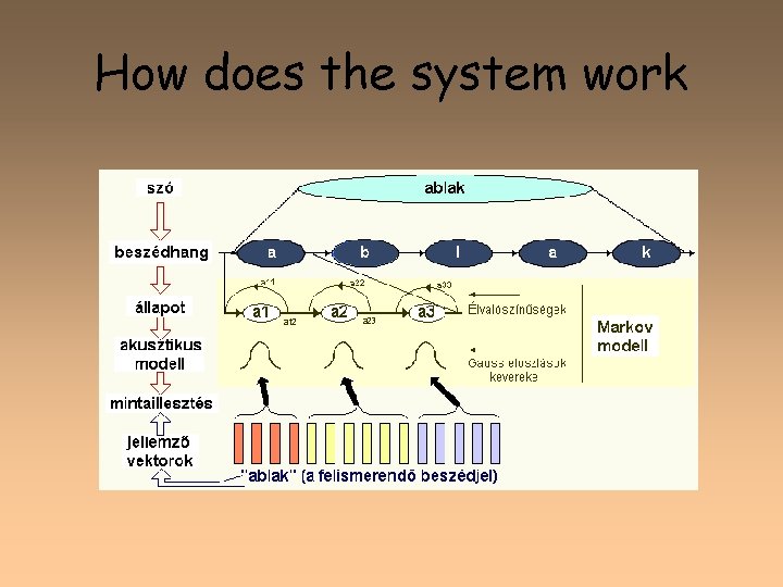
HMM in Speech Recognition

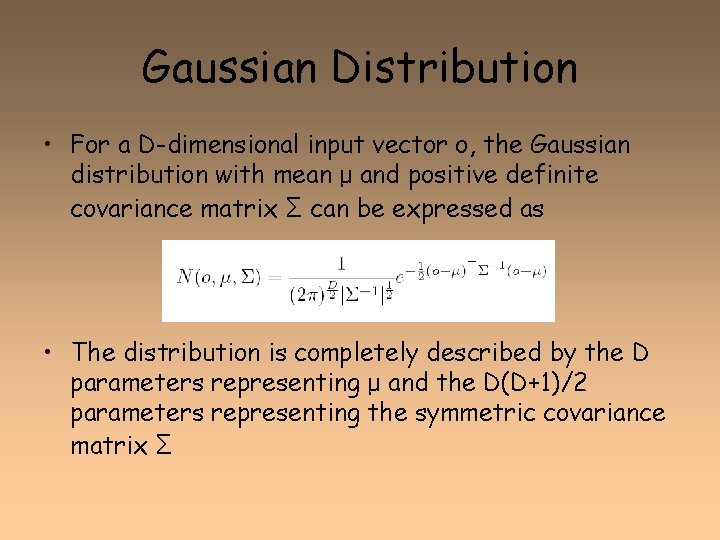
Gaussian Distribution • For a D-dimensional input vector o, the Gaussian distribution with mean μ and positive definite covariance matrix Σ can be expressed as • The distribution is completely described by the D parameters representing μ and the D(D+1)/2 parameters representing the symmetric covariance matrix Σ

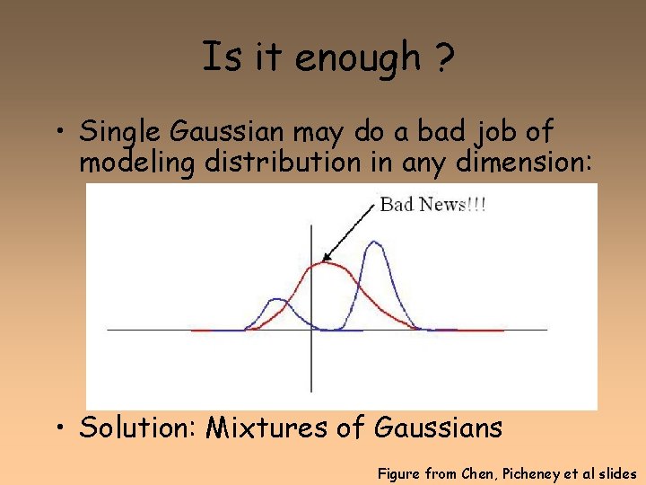
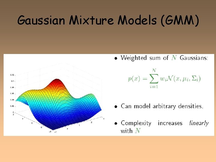
Is it enough ? • Single Gaussian may do a bad job of modeling distribution in any dimension: • Solution: Mixtures of Gaussians Figure from Chen, Picheney et al slides

Gaussian Mixture Models (GMM)

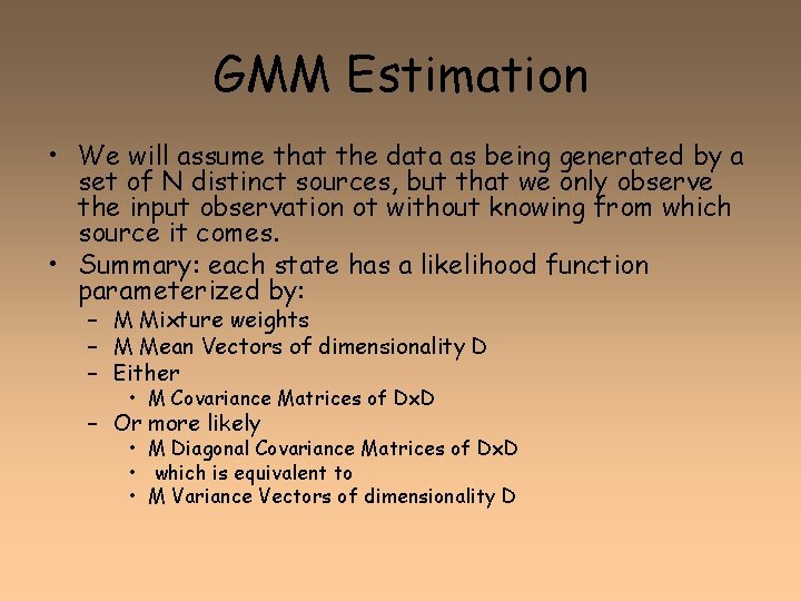
GMM Estimation • We will assume that the data as being generated by a set of N distinct sources, but that we only observe the input observation ot without knowing from which source it comes. • Summary: each state has a likelihood function parameterized by: – M Mixture weights – M Mean Vectors of dimensionality D – Either • M Covariance Matrices of Dx. D – Or more likely • M Diagonal Covariance Matrices of Dx. D • which is equivalent to • M Variance Vectors of dimensionality D

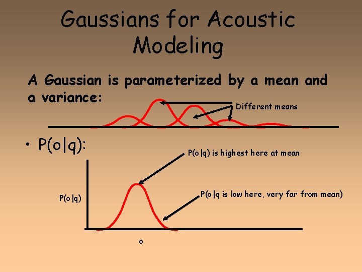
Gaussians for Acoustic Modeling A Gaussian is parameterized by a mean and a variance: Different means • P(o|q): P(o|q) is highest here at mean P(o|q is low here, very far from mean) P(o|q) o

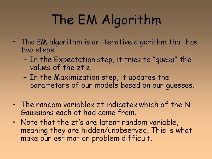
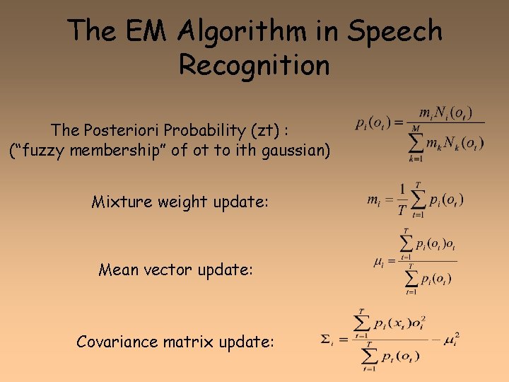
The EM Algorithm • The EM algorithm is an iterative algorithm that has two steps. – In the Expectation step, it tries to ”guess” the values of the zt’s. – In the Maximization step, it updates the parameters of our models based on our guesses. • The random variables zt indicates which of the N Gaussians each ot had come from. • Note that the zt’s are latent random variable, meaning they are hidden/unobserved. This is what make our estimation problem difficult.

The EM Algorithm in Speech Recognition The Posteriori Probability (zt) : (“fuzzy membership” of ot to ith gaussian) Mixture weight update: Mean vector update: Covariance matrix update:

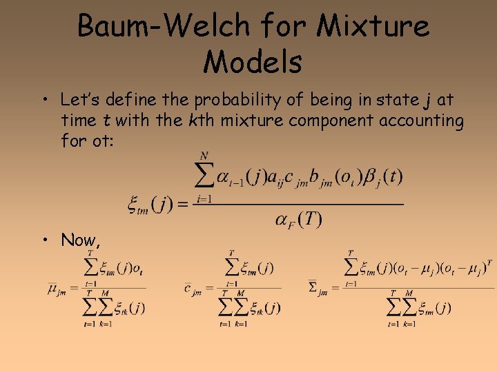
Baum-Welch for Mixture Models • Let’s define the probability of being in state j at time t with the kth mixture component accounting for ot: • Now,

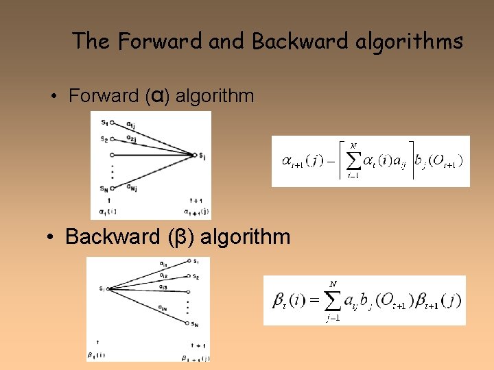
The Forward and Backward algorithms • Forward (α) algorithm • Backward (β) algorithm

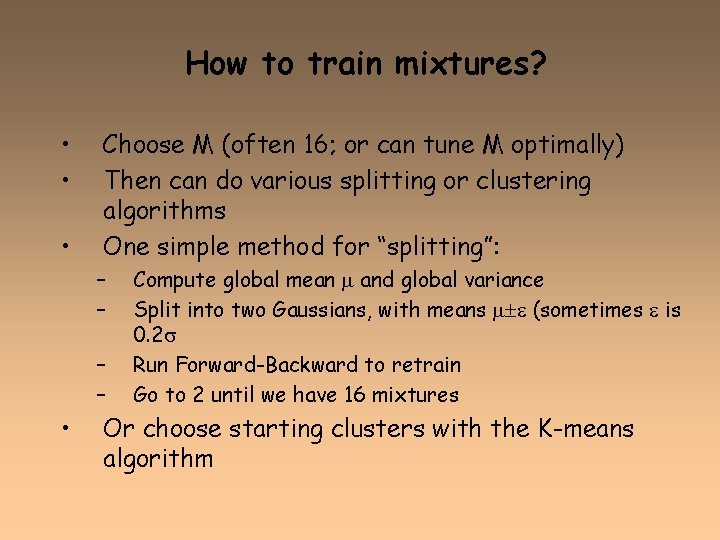
How to train mixtures? • • • Choose M (often 16; or can tune M optimally) Then can do various splitting or clustering algorithms One simple method for “splitting”: – – • Compute global mean and global variance Split into two Gaussians, with means (sometimes is 0. 2 Run Forward-Backward to retrain Go to 2 until we have 16 mixtures Or choose starting clusters with the K-means algorithm

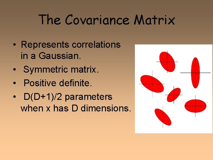
The Covariance Matrix • Represents correlations in a Gaussian. • Symmetric matrix. • Positive definite. • D(D+1)/2 parameters when x has D dimensions.

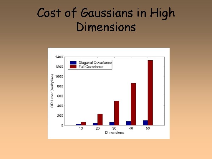
But: assume diagonal covariance • I. e. , assume that the features in the feature vector are uncorrelated • This isn’t true for FFT features, but is true for MFCC features. • Computation and storage much cheaper if diagonal covariance. • I. e. only diagonal entries are non-zero • Diagonal contains the variance of each dimension ii 2 • So this means we consider the variance of each acoustic feature (dimension) separately

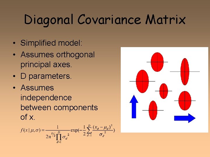
Diagonal Covariance Matrix • Simplified model: • Assumes orthogonal principal axes. • D parameters. • Assumes independence between components of x.

Cost of Gaussians in High Dimensions

How does the system work

References • Lawrence R. Rabiner - A Tutorial on Hidden Markov Models and Selected Aplivations in Speech Recognition • Magyar nyelvi beszédtechnológiai alapismeretek Multimédiás szoftver CD Nikol Kkt. 2002. • Dan Jurafsky – “CS Speech Recognition and Synthesis” Lecture 8 -10 Stanford University, 2005