Garbage Collection Terminology Heap a finite pool of

Garbage Collection

Terminology • Heap – a finite pool of data cells, can be organized in many ways • Roots - Pointers from the program into the Heap. – We must keep track of these. – All pointers from global varaibles – All pointers from temporarys (often on the stack) • Marking – Tracing the live data, starting at the roots. Leave behind a “mark” when we have visited a cell.

Things to keep in mind • Costs – How much does it cost as function of – All data – Just the live data • Overhead – Garbage collection is run when we have little or no space. What space does it require to run the collector? • Complexity – How can we tell we are doing the right thing?

Structure of the Heap Things to note in a Mark and sweep collector The Freelist The Roots Links from function closures Links from data (like pair or list) Constants
 (+ x 7)) (val x 45) (val")
Structure of the Heap (fun f (x) (+ x 7)) (val x 45) (val y (let (val x 6) (val y 2) in ( (a) (+ x (+ y a))))) (val z (pair 7 'c'))
) •")
Changes in the heap • Intermediate result computation – (@ f (fst z)) • Assignment to things • Garbage collection

Changes in the heap • • • Intermediate result computation Assignment to things – (: = y (pair 44 ‘a’)) Garbage collection

Garbage Collection

Mark and Sweep • Cells have room for several things beside data HCell a = Cell { mark: : (IORef Bool) , key : : Int , payload : : IORef a , alloc. Link: : IORef (HCell a) , all. Link: : HCell a } | Null. Cell • All cells start linked together on the free list • Allocation takes 1 (or more cells) from the free list • Garbage collection has two phases – Mark (trace all live data from the roots) – Sweep (visit every cell, and add unmarked cells to free list)
.")
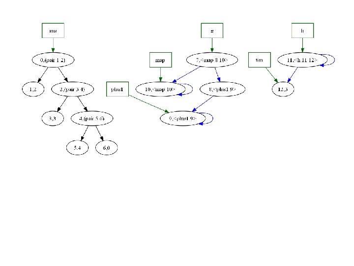
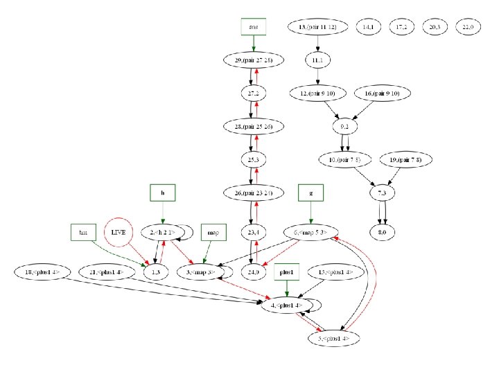
Mark phase (turns cells red in this picture).

Where do links into the heap reside? • In the environment interp. E : : -> -> -> Env (Range Value) State Exp IO(Value, State) -- the variables in scope -- the heap -- exp to interpret • Inside data values data Value = Int. V Int | Char. V Char | Con. V String Int (Range Value) | Fun. V Vname (Env (Range Value)) [Vname] Exp

Mark a cell mark. Cell mark. V Null. Cell = return Null. Cell mark. V (cell@(Cell m id p l 1 l 2)) = do { b <- read. IORef m; help b } where help True = return cell help False = do { write. IORef m True ; v <- read. IORef p ; v 2 <- mark. V (mark. Range mark. V) v ; write. IORef p v 2 ; return cell}
 Null. Cell = return (H all free)")
Sweeping through memory sweep (H all free) Null. Cell = return (H all free) sweep (H all free) (c@(Cell m id p l more)) = do { b <- read. IORef m ; if b then do { write. IORef m False ; sweep (H all free) more } else do { -- link it on the free write. IORef l free ; sweep (H all c) more }}
.")
Mark phase (turns cells red in this picture).

Two space collector • The heap is divided into two equal size regions • We allocate in the “active” region until no more space is left. • We trace the roots, creating an internal linked list of just the live data. • As we trace we compute where the cell will live in the new heap. • We forward all pointers to point in the new inactive region. • Flip the active and inactive regions

A heap Cell data HCell a = Cell { mark : : Mutable Bool , payload : : Mutable a , forward : : Mutable Addr , heaplink: : Mutable Addr , show. R: : a -> String }

The Heap data Heap a = Heap { heapsize : : Int , next. Active : : Addr , active : : (Array Int (HCell a)) , inactive: : (Array Int (HCell a)) , next. In. Active: : Mutable Addr , live. Link: : Mutable Addr }
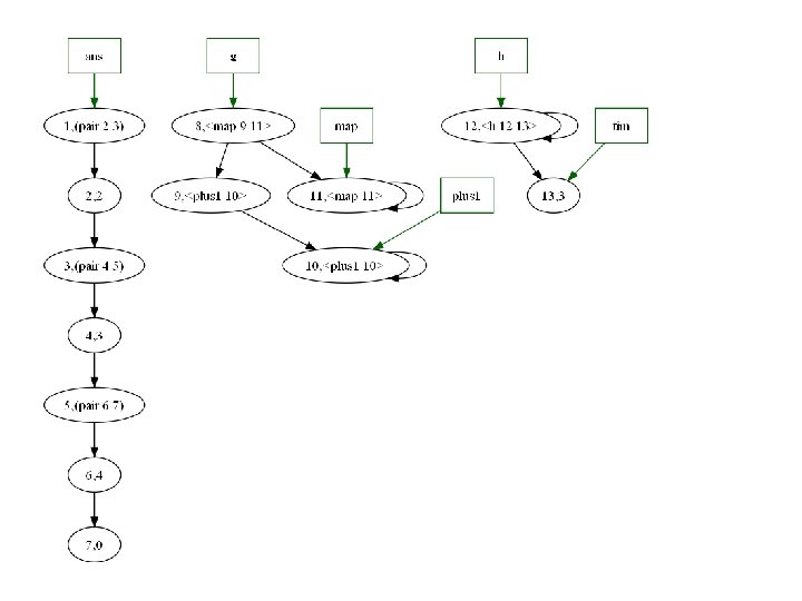
) (fun h (x) (+ x tim)) (fun map (f")
(val tim (+ 1 2)) (fun h (x) (+ x tim)) (fun map (f xs) (if (ispair xs) (pair (@ f (fst xs)) (@ map f (snd xs))) xs)) (fun plus 1 (x) (+ x 1)) (val g (@map plus 1)) (val ans (@g (pair 1 (pair 2 (pair 3 0)))) ) in ans { should yield (2. (3. (4. 0))) }
) (fun h (x) (+ x tim)) (fun map (f")
(val tim (+ 1 2)) (fun h (x) (+ x tim)) (fun map (f xs) (if (ispair xs) (pair (@ f (fst xs)) (@ map f (snd xs))) xs)) (fun plus 1 (x) (+ x 1)) (val g (@map plus 1)) (val ans (@g (pair 1 (pair 2 (pair 3 0)))) ) in ans { should yield (2. (3. (4. 0))) }
 -> Addr -> IO Addr mark. Addr (rec@(GCRec")
mark. Addr : : (GCRecord a) -> Addr -> IO Addr mark. Addr (rec@(GCRec heap markpay show. V )) index = mark cell where cell = active heap ! index next. Free. In. New. Heap = next. In. Active heap marked. List = live. Link heap mark (Cell m payld forward reachable showr) = do { mark <- read. IORef m ; if mark then do read. IORef forward else do { -- Set up recursive marking ; new <- fetch. And. Increment next. Free. In. New. Heap ; next <- read. IORef marked. List ; write. IORef marked. List index -- Update the fields of the cell, showing it is marked ; write. IORef m True ; write. IORef forward new ; write. IORef reachable next -- recursively mark the payload ; v <- read. IORef payld ; v 2 <- markpay (mark. Range rec) v -- copy payload in the inactive Heap with -- all payload pointers relocated. ; write. IORef (payload ((inactive heap) ! new)) v 2 -- finally return the Addr where this cell will be relocated to. ; return new }}

Kinds of collectors • • • Mark and sweep Two space collectors Relocating collectors Reference counting collectors Generational collectors

Reference counting collectors • Every cell contains a reference count. • It is incremented whenever a new pointer is added to a cell, and decremented whenever a pointer is changed from pointing at the cell to some other cell. • Cells whose reference counts drop to zero are garbage and are reclaimed.

Reference Counting • Advantages – Simple – Garbage is collected incrementally when it becomes free • Disadvantages – Circular structures are never collected – No upper bound on performing a pointer operation. (A cell may become free, and then all the cells it points to must be decremented, and they may become free) – Live cells become fragmented in memory (little spatial locality)

Generational Collectors • Assumptions – Most newly allocated cells become garbage quickly – Cells that survive 1 or 2 collections tend to be long lived – Old cells seldom (if ever) point to newer cells. – No need to spend time tracing pointers to old cells as one can assume that they are still reachable
 regions. • Each region holds cells of")
Strategy • Divide memory into (different sized) regions. • Each region holds cells of approximately the same age. • Allocate cells in the newest region (usually relatively small, often called the nursery) • When space in the newest region runs out, collect cells in only that region – Only trace the roots into the newest region – Assume everything in older regions is reachable • Special code to handle pointers from old regions to newer regions – Collect reachable cells in the newest region and promote them to an older region.

Program Roots backward pointers don’t need to be traced Most garbage is in the newest region. Only backward pointers within the collecting region need to be traced. Forward pointers into the collecting region must be handled just like program roots Forward pointers are rare

Generational Advantages Disadvantages • Small collection times • Code can be complex • Many forward pointers can wreck the otherwise good performance – Tracing only the live data – In only a (relatively small) region – No need to touch unreachable cells – Compacts live cells for better special locality

Other issues • Concurrent Collection – Separate processes – Race conditions – Approximate collection can be liveable • Finalization – When an object becomes garbage, it may free up other cells. Sometimes this can be done automatically, but other time specialized knowledge is needed. Finalizers allow programmers to add this knowledge

Overall Advantages of Garbage collectors • • Relieves programmers of an error prone task Removes dangling pointers Stops memory leaks Avoids “double frees” – Freeing a cell already freed (and subsequently reallocated) • Efficient implementation of “persistent” data structures – immutable data structures, can keep around old versions in case they are needed

Overall Disadvantages • Stop-the-world mentality – At any time the system may pause for GC • Timing and duration of GC times is unpredicatable • Unpredictable performance of the same code on the same data

Comparisons • Mark and trace is simple but can have long pauses. Tracing times are proportional to memory size • Reference Count systems are simple but can’t deal with cyclic structures, and all pointer manipulation operations can have unbounded upper limits • Two space collectors have times proportional to live memory. Can compact memory for better spatial locality, but use twice as much space.

Comparisons continued • Generational collectors can have the smallest pause times (proportional to live memory that is traced). Compact memory. With small nurserys don’t have as much spatial overhed as two space collectors. • Concurrent collectors. Run continuously. Code complicated to deal correctly with race conditions. Safe to leave some garbage uncollected if one can collect it later (when race conditions no longer apply).
- Slides: 35