Games and Adversarial Search CS 171 Fall 2016

Games and Adversarial Search CS 171, Fall 2016 Introduction to Artificial Intelligence Prof. Alexander Ihler

Types of games Deterministic: Chance: Perfect Information: chess, checkers, go, othello backgammon, monopoly Imperfect Information: battleship, Kriegspiel Bridge, poker, scrabble, … • Start with deterministic, perfect info games (easiest) • Not considered: – Physical games like tennis, ice hockey, etc. – But, see “robot soccer”, http: //www. robocup. org/

Typical assumptions • Two agents, whose actions alternate • Utility values for each agent are the opposite of the other – “Zero-sum” game; this creates adversarial situation • Fully observable environments • In game theory terms: – Deterministic, turn-taking, zero-sum, perfect information • Generalizes: stochastic, multiplayer, non zero-sum, etc. • Compare to e. g. , Prisoner’s Dilemma” (R&N pp. 666 -668) – Non-turn-taking, Non-zero-sum, Imperfect information

Game Tree (tic-tac-toe) • All possible moves at each step • How do we search this tree to find the optimal move?

Search versus Games • Search: no adversary – – Solution is (heuristic) method for finding goal Heuristics & CSP techniques can find optimal solution Evaluation function: estimate cost from start to goal through a given node Examples: path planning, scheduling activities, … • Games: adversary – Solution is a strategy • Specifices move for every possible opponent reply – Time limits force an approximate solution – Evaluation function: evaluate “goodness” of game position – Examples: chess, checkers, Othello, backgammon

Games as search • Two players, “MAX” and “MIN” • MAX moves first, & take turns until game is over – Winner gets reward, loser gets penalty – “Zero sum”: sum of reward and penalty is constant • Formal definition as a search problem: – – – Initial state: set-up defined by rules, e. g. , initial board for chess Player(s): which player has the move in state s Actions(s): set of legal moves in a state Results(s, a): transition model defines result of a move Terminal-Test(s): true if the game is finished; false otherwise Utility(s, p): the numerical value of terminal state s for player p • E. g. , win (+1), lose (-1), and draw (0) in tic-tac-toe • E. g. , win (+1), lose (0), and draw (1/2) in chess • MAX uses search tree to determine “best” next move

Min-Max: an optimal procedure • Designed to find the optimal strategy & best move for MAX: 1. Generate the whole game tree to leaves 2. Apply utility (payoff) function to leaves 3. Back-up values from leaves toward the root: • a Max node computes the max of its child values • a Min node computes the min of its child values 4. At root: choose move leading to the child of highest value

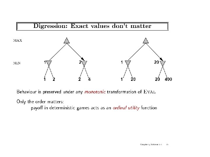
Two-ply Game Tree The minimax decision MAX MIN 3 3 3 12 2 2 8 2 4 6 14 5 2 Minimax maximizes the utility of the worst-case outcome for MAX

Recursive min-max search mm. Search(state) Simple stub to call recursion f’ns return argmax( [ min. Value( apply(state, a) ) for each action a ] ) max. Value(state) if (terminal(state)) return utility(state); v = -infty for each action a: v = max( v, min. Value( apply(state, a) ) ) return v min. Value(state) if (terminal(state)) return utility(state); v = infty for each action a: v = min( v, max. Value( apply(state, a) ) ) return v If recursion limit reached, eval position Otherwise, find our best child: If recursion limit reached, eval position Otherwise, find the worst child:

Properties of minimax • Complete? Yes (if tree is finite) • Optimal? – Yes (against an optimal opponent) – Can it be beaten by a suboptimal opponent? (No – why? ) • Time? O(bm) • Space? – O(bm) (depth-first search, generate all actions at once) – O(m) (backtracking search, generate actions one at a time)

Game tree size • Tic-tac-toe – B ¼ 5 legal actions per state on average; total 9 plies in game • “ply” = one action by one player; “move” = two plies – – 59 = 1, 953, 125 9! = 362, 880 (computer goes first) 8! = 40, 320 (computer goes second) Exact solution is quite reasonable • Chess – – B ¼ 35 (approximate average branching factor) D ¼ 100 (depth of game tree for “typical” game) Bd = 35100 ¼ 10154 nodes!!! Exact solution completely infeasible It is usually impossible to develop the whole search tree.

Cutting off search • One solution: cut off tree before game ends • Replace – Terminal(s) with Cutoff(s) – Utility(s, p) with Eval(s, p) – e. g. , stop at some max depth – estimate position quality • Does it work in practice? – – – Bm = 106, b = 35 ) m = 4 4 -ply lookahead is a poor chess player 4 -ply ¼ human novice 8 -ply ¼ typical PC, human master 12 -ply ¼ Deep Blue, Kasparov

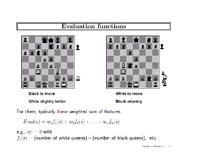
Static (Heuristic) Evaluation Functions • An Evaluation Function: – Estimate how good the current board configuration is for a player. – Typically, evaluate how good it is for the player, and how good it is for the opponent, and subtract the opponent’s score from the player’s. – Often called “static” because it is called on a static board position – Ex: Othello: Number of white pieces - Number of black pieces – Ex: Chess: Value of all white pieces - Value of all black pieces • Typical value ranges: [ -1, 1 ] (loss/win) or [ -1 , +1 ] or [ 0 , 1 ] • Board evaluation: X for one player ) -X for opponent – Zero-sum game: scores sum to a constant

Applying minimax to tic-tac-toe • The static heuristic evaluation function: – Count the number of possible win lines O X X O X has 6 possible win paths X has 4 possible wins O has 6 possible wins X has 5 possible wins O has 4 possible wins E(n) = 4 – 6 = -2 E(n) = 5 – 4 = 1 O O has 5 possible win paths E(s) = 6 – 5 = 1

Minimax values (two ply)

Minimax values (two ply)

Minimax values (two ply)

Iterative deepening • In real games, there is usually a time limit T to make a move • How do we take this into account? • Minimax cannot use “partial” results with any confidence, unless the full tree has been searched – Conservative: set small depth limit to guarantee finding a move in time < T – But, we may finish early – could do more search! • In practice, iterative deepening search (IDS) is used – IDS: depth-first search with increasing depth limit – When time runs out, use the solution from previous depth – With alpha-beta pruning (next), we can sort the nodes based on values from the previous depth limit in order to maximize pruning during the next depth limit ) search deeper!

Limited horizon effects • The Horizon Effect – Sometimes there’s a major “effect” (such as a piece being captured) which is just “below” the depth to which the tree has been expanded. – The computer cannot see that this major event could happen because it has a “limited horizon”. – There are heuristics to try to follow certain branches more deeply to detect such important events – This helps to avoid catastrophic losses due to “short-sightedness” • Heuristics for Tree Exploration – – Often better to explore some branches more deeply in the allotted time Various heuristics exist to identify “promising” branches Stop at “quiescent” positions – all battles are over, things are quiet Continue when things are in violent flux – the middle of a battle

Selectively deeper game trees 4 MAX (Computer’s move) MIN (Opponent’s move) 3 4 8 5 3 5 4 0 5 0 7 7 8

Eliminate redundant nodes • On average, each board position appears in the search tree approximately 10150 / 1040 = 10100 times – Vastly redundant search effort • Can’t remember all nodes (too many) – Can’t eliminate all redundant nodes • Some short move sequences provably lead to a redundant position – These can be deleted dynamically with no memory cost • Example: 1. P-QR 4; 2. P-KR 4 leads to the same position as 1. P-QR 4 P-KR 4; 2. P-KR 4 P-QR 4

Summary • Game playing as a search problem • Game trees represent alternate computer / opponent moves • Minimax: choose moves by assuming the opponent will always choose the move that is best for them – Avoids all worst-case outcomes for Max, to find the best – If opponent makes an error, Minimax will take optimal advantage (after) & make the best possible play that exploits the error • Cutting off search – – In general, it’s infeasible to search the entire game tree In practice, Cutoff-Test decides when to stop searching Prefer to stop at quiescent positions Prefer to keep searching in positions that are still in flux • Static heuristic evaluation function – Estimate the quality of a given board configuration for MAX player – Called when search is cut off, to determine value of position found

Games & Adversarial Search: Alpha-Beta Pruning CS 171, Fall 2016 Introduction to Artificial Intelligence Prof. Alexander Ihler

Alpha-Beta pruning • Exploit the “fact” of an adversary • If a position is provably bad – It’s no use searching to find out just how bad • If the adversary can force a bad position – It’s no use searching to find the good positions the adversary won’t let you achieve • Bad = not better than we can get elsewhere

Pruning with Alpha/Beta Do these nodes matter? If they = +1 million? If they = − 1 million?

Alpha-Beta Example Initially, possibilities are unknown: range (®=-1, ¯=+1) Do a depth-first search to the first leaf. ® = -1 ¯ = +1 Child inherits current ® and ¯ ® = -1 ¯ = +1 ? ? MAX ? ? MIN

Alpha-Beta Example See the first leaf, after MIN’s move: MIN updates ¯ ® = -1 ¯ = +1 MAX ® = -1 ¯=3 +1 · 3 ® < ¯ so no pruning ? ? 3 ? ? MIN

Alpha-Beta Example See remaining leaves; value is known Pass outcome to caller; MAX updates ® ® = -1 3 ¯ = +1 ¸ 3 ® = -1 ¯=3 3 3 12 ? ? 8 MAX ? ? MIN

Alpha-Beta Example Continue depth-first search to next leaf. Pass ®, ¯ to descendants ®=3 ¯ = +1 ¸ 3 MAX Child inherits current ® and ¯ ® = -1 ¯=3 ®=3 ¯ = +1 3 ? ? 3 12 8 ? ? MIN

Alpha-Beta Example Observe leaf value; MIN’s level; MIN updates beta Prune – play will never reach the other nodes! ®=3 ¯ = +1 ® ¸ ¯ !!! (what does this mean? ) ® = -1 ¯=3 ¸ 3 ®=3 ¯=2 +1. 3 MAX · 2 (This node is worse for MAX) 3 12 8 2 ? ? X ? ? Prune!!! MIN

Alpha-Beta Example Pass outcome to caller & update caller: ®=3 ¯ = +1 ¸ 3 MAX level, 3 ¸ 2 ) no change ® = -1 ¯=3 3 ®=3 ¯=2 12 8 2 · 2 X ? ? X MIN

Alpha-Beta Example Continue depth-first exploration… No pruning here; value is not resolved until final leaf. ®=3 ¯ = +1 ¸ 3 MAX Child inherits current ® and ¯ ® = -1 ¯=3 3 ®=3 ¯=2 12 8 2 ®=3 ¯ = +1 · 2 X X 14 MIN 2 5 2

Alpha-Beta Example Value at the root is resolved. ®=3 ¯ = +1 3 ® = -1 ¯=3 3 ®=3 ¯=2 12 8 2 Pass outcome to caller & update ®=3 ¯=2 · 2 X X 14 MIN 2 5 MAX 2

General alpha-beta pruning • Consider a node n in the tree: • If player has a better choice at – Parent node of n – Or, any choice further up! • Then n is never reached in play • So: – When that much is known about n, it can be pruned

Recursive ®-¯ pruning ab. Search(state) Simple stub to call recursion f’ns Initialize alpha, beta; no move found alpha, beta, a = -infty, +infty, None Score each action; update alpha & best action for each action a: alpha, a = max( (alpha, a) , (min. Value( apply(state, a), alpha, beta), a) ) return a max. Value(state, al, be) if (cutoff(state)) return eval(state); for each action a: al = max( al, min. Value( apply(state, a), al, be) if (al ¸ be) return +infty return al min. Value(state, al, be) if (cutoff(state)) return eval(state); for each action a: be = min( be, max. Value( apply(state, a), al, be) if (al ¸ be) return -infty return be If recursion limit reached, eval heuristic Otherwise, find our best child: If our options are too good, our min ancestor will never let us come this way Otherwise return the best we can find If recursion limit reached, eval heuristic Otherwise, find the worst child: If our options are too bad, our max ancestor will never let us come this way Otherwise return the worst we can find

Effectiveness of ®-¯ Search • Worst-Case – Branches are ordered so that no pruning takes place. In this case alpha-beta gives no improvement over exhaustive search • Best-Case – Each player’s best move is the left-most alternative (i. e. , evaluated first) – In practice, performance is closer to best rather than worst-case • In practice often get O(b(d/2)) rather than O(bd) – This is the same as having a branching factor of sqrt(b), • since (sqrt(b))d = b(d/2) (i. e. , we have effectively gone from b to square root of b) – In chess go from b ~ 35 to b ~ 6 • permiting much deeper search in the same amount of time

Iterative deepening • In real games, there is usually a time limit T to make a move • How do we take this into account? • Minimax cannot use “partial” results with any confidence, unless the full tree has been searched – Conservative: set small depth limit to guarantee finding a move in time < T – But, we may finish early – could do more search! • Added benefit with Alpha-Beta Pruning: – – – Remember node values found at the previous depth limit Sort current nodes so that each player’s best move is left-most child Likely to yield good Alpha-Beta Pruning ) better, faster search Only a heuristic: node values will change with the deeper search Usually works well in practice

Comments on alpha-beta pruning • Pruning does not affect final results • Entire subtrees can be pruned • Good move ordering improves pruning – Order nodes so player’s best moves are checked first • Repeated states are still possible – Store them in memory = transposition table

Iterative deepening reordering Which leaves can be pruned? None! MAX because the most favorable nodes are explored last… MIN 3 4 1 2 7 8 5 6

Iterative deepening reordering Different exploration order: now which leaves can be pruned? Lots! MAX because the most favorable nodes are explored first! MIN 6 5 8 7 2 1 3 4

Iterative deepening reordering Order with no pruning; use iterative deepening approach. Assume node score is the average of leaf values below. MAX 4. 5 L=0 MIN 3 4 1 2 7 8 5 6

Iterative deepening reordering Order with no pruning; use iterative deepening approach. Assume node score is the average of leaf values below. MAX For L=2, switch the order of these nodes! 6. 5 MIN 2. 5 L=1 3 4 6. 5 1 2 7 8 5 6

Iterative deepening reordering Order with no pruning; use iterative deepening approach. Assume node score is the average of leaf values below. MAX For L=2, switch the order of these nodes! 6. 5 MIN 6. 5 L=1 7 8 2. 5 5 6 3 4 1 2

Iterative deepening reordering Order with no pruning; use iterative deepening approach. Assume node score is the average of leaf values below. MAX Alpha-Beta pruning would prune this node at L=2 5. 5 MIN For L=3, switch the order of these nodes! L=2 5. 5 3. 5 7 3. 5 5. 5 8 5 6 3 4 1 2

Iterative deepening reordering Order with no pruning; use iterative deepening approach. Assume node score is the average of leaf values below. MAX Alpha-Beta pruning would prune this node at L=2 5. 5 MIN For L=3, switch the order of these nodes! L=2 5. 5 3. 5 7. 5 6 7 8 3 4 1 2

Iterative deepening reordering Order with no pruning; use iterative deepening approach. Assume node score is the average of leaf values below. MAX Lots of pruning! The most favorable nodes are explored earlier. 6 MIN 6 6 L=3 5 6 4 4 7 7 8 3 4 1 2

Longer Alpha-Beta Example Branch nodes are labelel A. . K for easy discussion =− , , initial values =+ MAX A E B F G 9 4 C H 4 MIN D I 9 J K 6 5 6 6 1 9 5 4 1 3 2 6 1 3 6 8 6 3 MAX

Longer Alpha-Beta Example Note that cut-off occurs at different depths… =− current , , =+ passed to kids MAX =− =+ kid=A A B C D =− =+ kid=E E F G 9 4 H 4 I 9 MIN J K 6 5 6 6 1 9 5 4 1 3 2 6 1 3 6 8 6 3 MAX

Longer Alpha-Beta Example =− =+ see first leaf, MAX updates MAX =− =+ kid=A =4 =+ kid=E E 4 4 4 A B F C G 9 H 4 MIN D I 9 J K 6 5 6 6 1 9 5 4 1 3 2 6 1 3 6 8 6 3 We also are running Mini. Max search and recording node values within the triangles, without explicit comment. MAX

Longer Alpha-Beta Example =− =+ see next leaf, MAX updates MAX =− =+ kid=A =5 =+ kid=E E 5 A B F C G 9 H 4 MIN D I 9 J K 6 5 4 5 6 6 1 9 5 4 1 3 2 6 1 3 6 8 6 3 MAX

Longer Alpha-Beta Example =− =+ see next leaf, MAX updates MAX =− =+ kid=A =6 =+ kid=E E B F 6 6 4 A C G 9 H 4 MIN D I 9 J K 6 5 6 6 1 9 5 4 1 3 2 6 1 3 6 8 6 3 MAX

Longer Alpha-Beta Example =− =+ return node value, MIN updates MAX =− =6 kid=A A 6 B C MIN D 6 E 6 F G 9 4 H 4 I 9 J K 6 5 6 6 1 9 5 4 1 3 2 6 1 3 6 8 6 3 MAX

Longer Alpha-Beta Example current , , passed to kid F =− =+ MAX =− =6 kid=A =− =6 kid=F E 6 A 6 F C G 9 4 B H 4 MIN D I 9 J K 6 5 6 6 1 9 5 4 1 3 2 6 1 3 6 8 6 3 MAX

Longer Alpha-Beta Example =− =+ see first leaf, MAX updates MAX =− =6 kid=A =6 =6 kid=F E F 6 6 4 A 6 B C G 6 9 H 4 MIN D I 9 J K 6 5 6 6 1 9 5 4 1 3 2 6 1 3 6 8 6 3 MAX

Longer Alpha-Beta Example α β !! Prune!! =− =+ MAX =− =6 kid=A =6 =6 kid=F E 6 A 6 F B G 6 9 4 C XX H 4 MIN D I 9 J K 6 5 6 6 1 9 5 4 1 3 2 6 1 3 6 8 6 3 MAX

Longer Alpha-Beta Example =− return node value, =+ MIN updates , no change to =− =6 kid=A A 6 B MAX C MIN D 6 E 6 F G 6 9 4 XX H 4 I 9 J K MAX 6 5 6 6 1 9 5 4 1 3 2 6 1 3 6 8 6 3 If we had continued searching at node F, we would see the 9 from its third leaf. Our returned value would be 9 instead of 6. But at A, MIN would choose E(=6) instead of F(=9). I nternal values may change; root values do not.

Longer Alpha-Beta Example =− =+ see next leaf, MIN updates , no change to =− =6 kid=A MAX A 6 B C MIN D 9 E 6 F G 6 9 4 XX H 4 I 9 J K 6 5 6 6 1 9 5 4 1 3 2 6 1 3 6 8 6 3 MAX

Longer Alpha-Beta Example =6 =+ return node value, MAX updates α 6 MAX 6 A 6 E 6 F B G 6 9 4 C XX H 4 MIN D I 9 J K 6 5 6 6 1 9 5 4 1 3 2 6 1 3 6 8 6 3 MAX

Longer Alpha-Beta Example current , , passed to kids =6 =+ =6 =+ kid=B =6 =+ kid=G E 6 A 6 F B 9 4 XX MAX C G 6 6 H 4 MIN D I 9 J K 6 5 6 6 1 9 5 4 1 3 2 6 1 3 6 8 6 3 MAX

Longer Alpha-Beta Example =6 =+ see first leaf, MAX updates , no change to =6 =+ kid=B =6 =+ kid=G E 6 A 6 F B G 6 9 4 6 XX MAX C H 5 4 MIN D I 9 J K 6 5 5 6 6 1 9 5 4 1 3 2 6 1 3 6 8 6 3 MAX

Longer Alpha-Beta Example =6 =+ see next leaf, MAX updates , no change to =6 =+ kid=B =6 =+ kid=G E 6 A 6 F B G 6 6 9 MAX C H 5 4 MIN D I 9 J K 6 4 4 XX 5 6 6 1 9 5 4 1 3 2 6 1 3 6 8 6 3 MAX

Longer Alpha-Beta Example =6 =+ return node value, MIN updates =6 =5 kid=B A 6 6 B 5 MAX C MIN D 5 E 6 F G 6 9 4 XX H 5 4 I 9 J K 6 5 6 6 1 9 5 4 1 3 2 6 1 3 6 8 6 3 MAX

Longer Alpha-Beta Example α β !! Prune!! =6 =+ =6 =5 kid=B E 6 A 6 F B 5 G 6 9 4 6 XX 5 MAX C H I ? 4 X 9 XX MIN D J K 6 5 6 6 1 9 5 4 1 3 2 6 1 3 6 8 6 3 Note that we never find out, what is the node value of H? But we have proven it doesn ’t matter, so we don’t care. MAX

Longer Alpha-Beta Example =6 =+ return node value, MAX updates α, no change to α 6 MAX 5 A 6 E 6 F B 5 G 6 9 4 XX 5 C H I ? 4 X 9 XX MIN D J K 6 5 6 6 1 9 5 4 1 3 2 6 1 3 6 8 6 3 MAX

Longer Alpha-Beta Example current , , passed to kid=C =6 =+ =6 =+ kid=C E 6 A 6 F B 5 G 6 9 4 6 XX 5 MAX C H I ? 4 X 9 XX MIN D J K 6 5 6 6 1 9 5 4 1 3 2 6 1 3 6 8 6 3 MAX

Longer Alpha-Beta Example =6 =+ see first leaf, MIN updates =6 =9 kid=C A 6 6 B 5 MAX C 9 MIN D 9 E 6 F G 6 9 4 XX 5 H I ? 4 X 9 XX J K 6 5 6 6 1 9 5 4 1 3 2 6 1 3 6 8 6 3 MAX

Longer Alpha-Beta Example current , , passed to kid I =6 =+ =6 =9 kid=C =6 =9 kid=I E 6 A 6 F B 5 G 6 9 4 6 XX 5 MAX C 9 H I ? 4 X 9 XX MIN D J K 6 5 6 6 1 9 5 4 1 3 2 6 1 3 6 8 6 3 MAX

Longer Alpha-Beta Example =6 =+ see first leaf, MAX updates , no change to =6 =9 kid=C =6 =9 kid=I E 6 A 6 F B 5 G 6 6 9 5 MAX C 9 H I 2 ? 4 X 9 MIN D J K 6 2 4 XX XX 5 6 6 1 9 5 4 1 3 2 6 1 3 6 8 6 3 MAX

Longer Alpha-Beta Example =6 =+ see next leaf, MAX updates , no change to =6 =9 kid=C =6 =9 kid=I E 6 A 6 F B 5 G 6 9 4 6 XX 5 MAX C 9 H I 6 ? 4 X 9 XX MIN D J 6 K 6 5 6 6 1 9 5 4 1 3 2 6 1 3 6 8 6 3 MAX

Longer Alpha-Beta Example =6 =+ return node value, MIN updates β =6 =6 kid=C A 6 6 B 5 MAX C 6 MIN D 6 E 6 F G 6 9 4 XX 5 H I 6 ? 4 X 9 XX J K 6 5 6 6 1 9 5 4 1 3 2 6 1 3 6 8 6 3 MAX

Longer Alpha-Beta Example α β !! Prune!! =6 =+ =6 =6 kid=C E 6 A 6 F B 5 G 6 9 4 6 XX 5 MAX C 6 H I ? 4 X D 6 MIN J ? 9 XX K 6 X XX 5 6 6 1 9 5 4 1 3 2 6 1 3 6 8 6 3 MAX

Longer Alpha-Beta Example =6 =+ return node value, MAX updates α, no change to α 6 MAX 6 A 6 E 6 F B 5 G 6 9 4 XX 5 C 6 H I ? 4 X MIN D 6 J 9 XX K ? 6 X XX 5 6 6 1 9 5 4 1 3 2 6 1 3 6 8 6 3 MAX

Longer Alpha-Beta Example current , , passed to kid=D =6 =+ =6 =+ kid=D E 6 A 6 F B 5 G 6 9 4 6 XX 5 MAX C 6 H I ? 4 X MIN D 6 J 9 XX K ? 6 X XX 5 6 6 1 9 5 4 1 3 2 6 1 3 6 8 6 3 MAX

Longer Alpha-Beta Example =6 =+ see first leaf, MIN updates =6 =6 kid=D E 6 A 6 F B 5 G 6 9 4 6 XX 5 MAX C 6 H I ? 4 X D 6 6 MIN J 6 9 XX K ? 6 X XX 5 6 6 1 9 5 4 1 3 2 6 1 3 6 8 6 3 MAX

Longer Alpha-Beta Example α β !! Prune!! =6 =+ =6 =6 kid=D E 6 A 6 F B 5 G 6 9 4 6 XX 5 MAX C 6 H I ? 4 X 9 XX D 6 6 MIN J K ? ? MAX 6 X XX XX X 5 6 6 1 9 5 4 1 3 2 6 1 3 6 8 6 3

Alpha-Beta Example #2 return node value, =6 =+ MAX updates α, 6 no change to α MAX 6 A 6 E 6 F B 5 G 6 9 4 XX 5 C 6 H I ? 4 X 9 XX D 6 6 MIN J K ? ? MAX 6 X XX XX X 5 6 6 1 9 5 4 1 3 2 6 1 3 6 8 6 3

Alpha-Beta Example #2 MAX moves to A, and expects to get 6 6 MAX’s move A 6 E 6 F B 5 G 6 9 4 XX 5 MAX C 6 H I ? 4 X 9 XX D 6 6 MIN J K ? ? MAX 6 X XX XX X 5 6 6 1 9 5 4 1 3 2 6 1 3 6 8 6 3 Although we may have changed some internal branch node return values, the final root action and expected outcome are identical to if we had not done alpha-beta pruning. I nternal values may change; root values do not.

Nondeterministic games • Ex: Backgammon – Roll dice to determine how far to move (random) – Player selects which checkers to move (strategy) https: //commons. wikimedia. org/wiki/File: Backgammon_lg. jpg

Nondeterministic games • Chance (random effects) due to dice, card shuffle, … • Chance nodes: expectation (weighted average) of successors • Simplified example: coin flips MAX’s move MAX 3 “Expectiminimax” 0. 5 2 2 3 -1 0. 5 4 4 7 0. 5 0 4 6 Chance -2 0 5 MIN -2

Pruning in nondeterministic games • Can still apply a form of alpha-beta pruning 3 MAX 3 0. 5 2 2 -1 0. 5 4 4 7 0. 5 0 4 6 Chance -2 0 5 MIN -2

Pruning in nondeterministic games • Can still apply a form of alpha-beta pruning (-1, 1) MAX (-1, 1) 3 0. 5 3 -1 0. 5 (-1, 1) Chance 0. 5 (-1, 1) MIN 2 4 7 4 6 0 5 -2

Pruning in nondeterministic games • Can still apply a form of alpha-beta pruning (-1, 1) (-1, 2) MAX (-1, 1) 3 0. 5 3 -1 0. 5 (-1, 1) Chance 0. 5 (-1, 1) MIN 2 4 7 4 6 0 5 -2

Pruning in nondeterministic games • Can still apply a form of alpha-beta pruning (-1, 1) (2, 2) MAX (-1, 1) 3 0. 5 3 -1 0. 5 (-1, 1) Chance 0. 5 (-1, 1) MIN 2 4 7 4 6 0 5 -2

Pruning in nondeterministic games • Can still apply a form of alpha-beta pruning (-1, 1) (-1, 4. 5) (2, 2) MAX (-1, 1) 3 0. 5 3 -1 0. 5 (-1, 7) (-1, 1) Chance 0. 5 (-1, 1) MIN 2 4 7 4 6 0 5 -2

Pruning in nondeterministic games • Can still apply a form of alpha-beta pruning (3, 1) (3, 3) 0. 5 (2, 2) 3 MAX (-1, 1) 3 -1 0. 5 (4, 4) (-1, 1) Chance 0. 5 (-1, 1) MIN 2 4 7 4 6 0 5 -2

Pruning in nondeterministic games • Can still apply a form of alpha-beta pruning (3, 1) (3, 3) 0. 5 (2, 2) 3 MAX (-1, 1) 3 -1 0. 5 (4, 4) (-1, 6) Chance 0. 5 (-1, 1) MIN 2 4 7 4 6 0 5 -2

Pruning in nondeterministic games • Can still apply a form of alpha-beta pruning (3, 1) (3, 3) 0. 5 (2, 2) 3 MAX (-1, 1) 3 -1 0. 5 (4, 4) (0, 0) Chance 0. 5 (-1, 1) MIN 2 4 7 4 6 0 5 -2

Pruning in nondeterministic games • Can still apply a form of alpha-beta pruning (3, 1) (3, 3) 0. 5 (2, 2) 3 MAX (-1, 2. 5) 3 -1 0. 5 (4, 4) (0, 0) Chance 0. 5 (-1, 5) MIN 2 4 7 4 6 0 5 X-2 Prune!

Partially observable games • R&N Chapter 5. 6 – “The fog of war” • Background: R&N, Chapter 4. 3 -4 – Searching with Nondeterministic Actions/Partial Observations • Search through Belief States (see Fig. 4. 14) – Agent’s current belief about which states it might be in, given the sequence of actions & percepts to that point • Actions(b) = ? ? Union? Intersection? – Tricky: an action legal in one state may be illegal in another – Is an illegal action a NO-OP? or the end of the world? • Transition Model: – Result(b, a) = { s’ : s’ = Result(s, a) and s is a state in b } • Goaltest(b) = every state in b is a goal state

Belief States for Unobservable Vacuum World 103

Partially observable games • • R&N Chapter 5. 6 Player’s current node is a belief state Player’s move (action) generates child belief state Opponent’s move is replaced by Percepts(s) – Each possible percept leads to the belief state that is consistent with that percept • Strategy = a move for every possible percept sequence • Minimax returns the worst state in the belief state • Many more complications and possibilities!! – Opponent may select a move that is not optimal, but instead minimizes the information transmitted, or confuses the opponent – May not be reasonable to consider ALL moves; open P-QR 3? ? • See R&N, Chapter 5. 6, for more info

The State of Play • Checkers: – Chinook ended 40 -year-reign of human world champion Marion Tinsley in 1994. • Chess: – Deep Blue defeated human world champion Garry Kasparov in a six-game match in 1997. • Othello: – human champions refuse to compete against computers: they are too good. • Go: – Alpha. Go recently (3/2016) beat 9 th dan Lee Sedol – b > 300 (!); full game tree has > 10^760 leaf nodes (!!) • See (e. g. ) http: //www. cs. ualberta. ca/~games/ for more info

High branching factors • What can we do when the search tree is too large? – Ex: Go ( b = 50 -200+ moves per state) – Heuristic state evaluation (score a partial game) • Where does this heuristic come from? – Hand designed – Machine learning on historical game patterns – Monte Carlo methods – play random games

Monte Carlo heuristic scoring • Idea: play out the game randomly, and use the results as a score – Easy to generate & score lots of random games – May use 1000 s of games for a node • The basis of Monte Carlo tree search algorithms… Image from www. mcts. ai

Monte Carlo Tree Search • Should we explore the whole (top of) the tree? – Some moves are obviously not good… – Should spend time exploring / scoring promising ones • This is a multi-armed bandit problem: • Want to spend our time on good moves • Which moves have high payout? – Hard to tell – random… • Explore vs. exploit tradeoff Image from Microsoft Research

Visualizing MCTS • At each level of the tree, keep track of – Number of times we’ve explored a path – Number of times we won • Follow winning (from max/min perspective) strategies more often, but also explore others

MCTS 1/1 MAB strategy 1/1 Default / random strategy Score consists of (1) % wins (2) # times tried (3) # of steps total UCT: Terminal state

MCTS 1/2 MAB strategy 1/1 Default / random strategy 0/1 Score consists of (1) % wins (2) # times tried (3) # of steps total UCT: Terminal state

MCTS 1/3 MAB strategy 1/2 0/1 Default / random strategy 0/1 Score consists of (1) % wins (2) # times tried (3) # of steps total UCT: Terminal state

Summary • Game playing is best modeled as a search problem • Game trees represent alternate computer/opponent moves • Evaluation functions estimate the quality of a given board configuration for the Max player. • Minimax is a procedure which chooses moves by assuming that the opponent will always choose the move which is best for them • Alpha-Beta is a procedure which can prune large parts of the search tree and allow search to go deeper • For many well-known games, computer algorithms based on heuristic search match or out-perform human world experts.