GamePlaying Adversarial Search This lecture topic GamePlaying Adversarial

Game-Playing & Adversarial Search This lecture topic: Game-Playing & Adversarial Search (two lectures) Chapter 5. 1 -5. 5 Next lecture topic: Constraint Satisfaction Problems (two lectures) Chapter 6. 1 -6. 4, except 6. 3. 3 (Please read lecture topic material before and after each lecture on that topic)

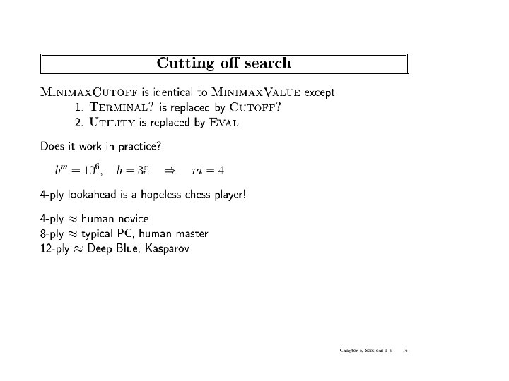
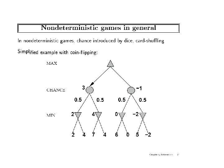
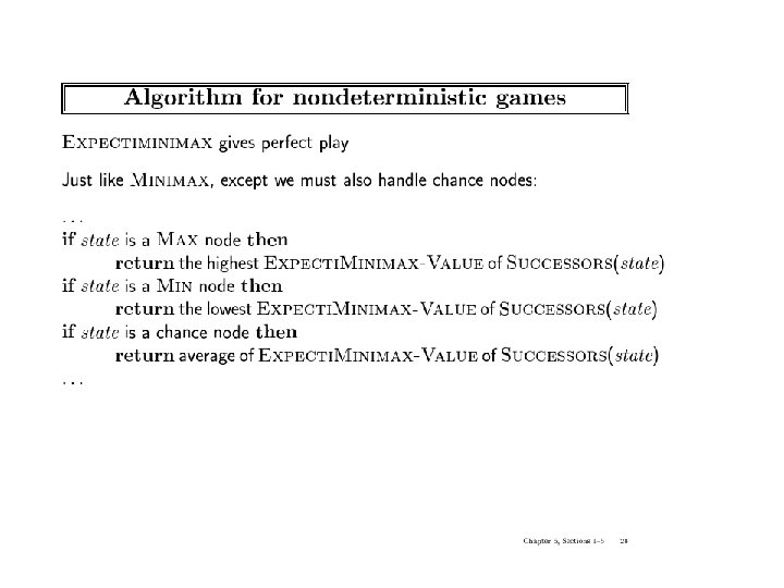
Overview • Minimax Search with Perfect Decisions – Impractical in most cases, but theoretical basis for analysis • Minimax Search with Cut-off – Replace terminal leaf utility by heuristic evaluation function • Alpha-Beta Pruning – The fact of the adversary leads to an advantage in search! • Practical Considerations – Redundant path elimination, look-up tables, etc. • Game Search with Chance – Expectiminimax search

You Will Be Expected to Know • Basic definitions (section 5. 1) • Minimax optimal game search (5. 2) • Alpha-beta pruning (5. 3) • Evaluation functions, cutting off search (5. 4. 1, 5. 4. 2) • Expectiminimax (5. 5)

Types of Games battleship Kriegspiel Not Considered: Physical games like tennis, croquet, ice hockey, etc. (but see “robot soccer” http: //www. robocup. org/)

Typical assumptions • Two agents whose actions alternate • Utility values for each agent are the opposite of the other – This creates the adversarial situation • Fully observable environments • In game theory terms: – “Deterministic, turn-taking, zero-sum games of perfect information” • Generalizes to stochastic games, multiple players, non zero-sum, etc. • Compare to, e. g. , “Prisoner’s Dilemma” (p. 666 -668, R&N 3 rd ed. ) – “Deterministic, NON-turn-taking, NON-zero-sum game of IMperfect information”

Game tree (2 -player, deterministic, turns) How do we search this tree to find the optimal move?

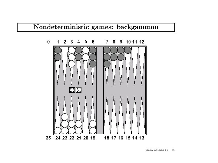
Search versus Games • Search – no adversary – – • Solution is (heuristic) method for finding goal Heuristics and CSP techniques can find optimal solution Evaluation function: estimate of cost from start to goal through given node Examples: path planning, scheduling activities Games – adversary – Solution is strategy • strategy specifies move for every possible opponent reply. – Time limits force an approximate solution – Evaluation function: evaluate “goodness” of game position – Examples: chess, checkers, Othello, backgammon

Games as Search • Two players: MAX and MIN • MAX moves first and they take turns until the game is over – Winner gets reward, loser gets penalty. – “Zero sum” means the sum of the reward and the penalty is a constant. • Formal definition as a search problem: – – – – • Initial state: Set-up specified by the rules, e. g. , initial board configuration of chess. Player(s): Defines which player has the move in a state. Actions(s): Returns the set of legal moves in a state. Result(s, a): Transition model defines the result of a move. (2 nd ed. : Successor function: list of (move, state) pairs specifying legal moves. ) Terminal-Test(s): Is the game finished? True if finished, false otherwise. Utility function(s, p): Gives numerical value of terminal state s for player p. • E. g. , win (+1), lose (-1), and draw (0) in tic-tac-toe. • E. g. , win (+1), lose (0), and draw (1/2) in chess. MAX uses search tree to determine next move.

An optimal procedure: The Min-Max method Designed to find the optimal strategy for Max and find best move: • 1. Generate the whole game tree, down to the leaves. • 2. Apply utility (payoff) function to each leaf. • 3. Back-up values from leaves through branch nodes: – a Max node computes the Max of its child values – a Min node computes the Min of its child values • 4. At root: choose the move leading to the child of highest value.

Game Trees

Two-Ply Game Tree

Two-Ply Game Tree

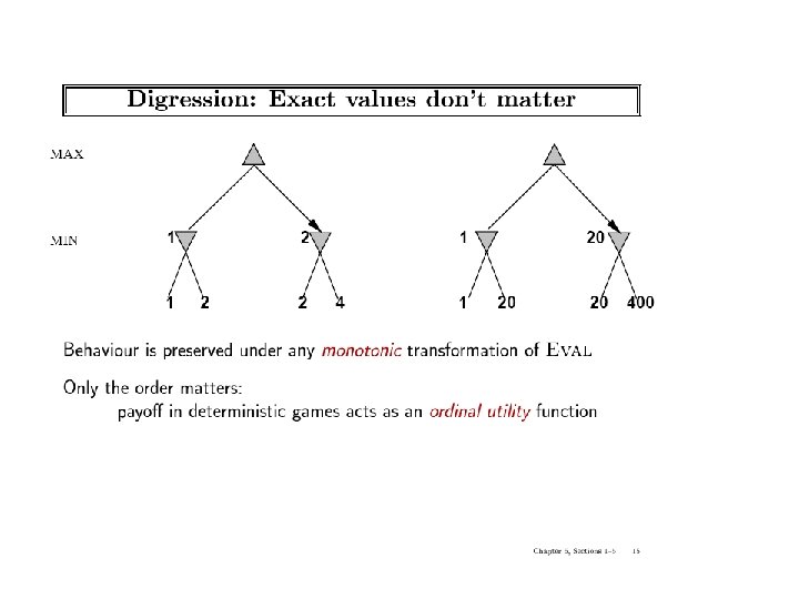
Two-Ply Game Tree Minimax maximizes the utility for the worst-case outcome for max The minimax decision

Pseudocode for Minimax Algorithm function MINIMAX-DECISION(state) returns an action inputs: state, current state in game return arg maxa ACTIONS(state) MIN-VALUE(Result(state, a)) function MAX-VALUE(state) returns a utility value if TERMINAL-TEST(state) then return UTILITY(state) v −∞ for a in ACTIONS(state) do v MAX(v, MIN-VALUE(Result(state, a))) return v function MIN-VALUE(state) returns a utility value if TERMINAL-TEST(state) then return UTILITY(state) v +∞ for a in ACTIONS(state) do v MIN(v, MAX-VALUE(Result(state, a))) return v

Properties of minimax • Complete? – Yes (if tree is finite). • Optimal? – Yes (against an optimal opponent). – Can it be beaten by an opponent playing sub-optimally? • No. (Why not? ) • Time complexity? – O(bm) • Space complexity? – O(bm) (depth-first search, generate all actions at once) – O(m) (backtracking search, generate actions one at a time)

Game Tree Size • Tic-Tac-Toe – b ≈ 5 legal actions per state on average, total of 9 plies in game. • “ply” = one action by one player, “move” = two plies. – 59 = 1, 953, 125 – 9! = 362, 880 (Computer goes first) – 8! = 40, 320 (Computer goes second) exact solution quite reasonable • Chess – b ≈ 35 (approximate average branching factor) – d ≈ 100 (depth of game tree for “typical” game) – bd ≈ 35100 ≈ 10154 nodes!! exact solution completely infeasible • It is usually impossible to develop the whole search tree.

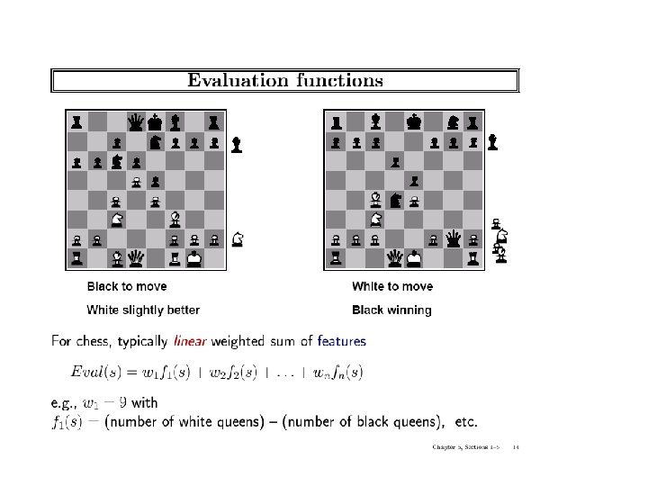
Static (Heuristic) Evaluation Functions • An Evaluation Function: – Estimates how good the current board configuration is for a player. – Typically, evaluate how good it is for the player, how good it is for the opponent, then subtract the opponent’s score from the player’s. – Othello: Number of white pieces - Number of black pieces – Chess: Value of all white pieces - Value of all black pieces • Typical values from -infinity (loss) to +infinity (win) or [-1, +1]. • If the board evaluation is X for a player, it’s -X for the opponent – “Zero-sum game”

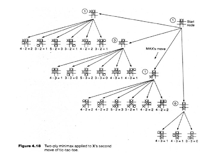
Applying Mini. Max to tic-tac-toe • The static evaluation function heuristic

Backup Values

Alpha-Beta Pruning Exploiting the Fact of an Adversary • If a position is provably bad: – It is NO USE expending search time to find out exactly how bad • If the adversary can force a bad position: – It is NO USE expending search time to find out the good positions that the adversary won’t let you achieve anyway • Bad = not better than we already know we can achieve elsewhere. • Contrast normal search: – ANY node might be a winner. – ALL nodes must be considered. – (A* avoids this through knowledge, i. e. , heuristics)

Tic-Tac-Toe Example with Alpha-Beta Pruning Backup Values

Another Alpha-Beta Example Do DF-search until first leaf Range of possible values [-∞, +∞]

Alpha-Beta Example (continued) [-∞, +∞] [-∞, 3]

Alpha-Beta Example (continued) [-∞, +∞] [-∞, 3]

Alpha-Beta Example (continued) [3, +∞] [3, 3]

Alpha-Beta Example (continued) [3, +∞] This node is worse for MAX [3, 3] [-∞, 2]

Alpha-Beta Example (continued) [3, 14] [3, 3] [-∞, 2] , [-∞, 14]

Alpha-Beta Example (continued) [3, 5] [3, 3] [−∞, 2] , [-∞, 5]

Alpha-Beta Example (continued) [3, 3] [−∞, 2] [2, 2]

Alpha-Beta Example (continued) [3, 3] [-∞, 2] [2, 2]

General alpha-beta pruning • Consider a node n in the tree --- • If player has a better choice at: – Parent node of n – Or any choice point further up • Then n will never be reached in play. • Hence, when that much is known about n, it can be pruned.

Alpha-beta Algorithm • Depth first search – only considers nodes along a single path from root at any time = highest-value choice found at any choice point of path for MAX (initially, = −infinity) = lowest-value choice found at any choice point of path for MIN (initially, = +infinity) • • • Pass current values of and down to child nodes during search. Update values of and during search: – MAX updates at MAX nodes – MIN updates at MIN nodes Prune remaining branches at a node when ≥

When to Prune • Prune whenever ≥ . – Prune below a Max node whose alpha value becomes greater than or equal to the beta value of its ancestors. • Max nodes update alpha based on children’s returned values. – Prune below a Min node whose beta value becomes less than or equal to the alpha value of its ancestors. • Min nodes update beta based on children’s returned values.

Alpha-Beta Example Revisited Do DF-search until first leaf , , initial values =− =+ , , passed to kids =− =+

Alpha-Beta Example (continued) =− =+ =− =3 MIN updates , based on kids

Alpha-Beta Example (continued) =− =+ =− =3 MIN updates , based on kids. No change.

Alpha-Beta Example (continued) MAX updates , based on kids. =3 =+ 3 is returned as node value.

Alpha-Beta Example (continued) =3 =+ , , passed to kids =3 =+

Alpha-Beta Example (continued) =3 =+ MIN updates , based on kids. =3 =2

Alpha-Beta Example (continued) =3 =+ =3 =2 ≥ , so prune.

Alpha-Beta Example (continued) MAX updates , based on kids. No change. =3 =+ 2 is returned as node value.

Alpha-Beta Example (continued) =3 =+ , , , passed to kids =3 =+

Alpha-Beta Example (continued) =3 =+ , MIN updates , based on kids. =3 =14

Alpha-Beta Example (continued) =3 =+ , MIN updates , based on kids. =3 =5

Alpha-Beta Example (continued) =3 =+ 2 is returned as node value. 2

Alpha-Beta Example (continued) Max calculates the same node value, and makes the same move! 2

Effectiveness of Alpha-Beta Search • Worst-Case – branches are ordered so that no pruning takes place. In this case alpha-beta gives no improvement over exhaustive search • Best-Case – each player’s best move is the left-most child (i. e. , evaluated first) – in practice, performance is closer to best rather than worst-case – E. g. , sort moves by the remembered move values found last time. – E. g. , expand captures first, then threats, then forward moves, etc. – E. g. , run Iterative Deepening search, sort by value last iteration. • In practice often get O(b(d/2)) rather than O(bd) – this is the same as having a branching factor of sqrt(b), • (sqrt(b))d = b(d/2), i. e. , we effectively go from b to square root of b – e. g. , in chess go from b ~ 35 to b ~ 6 • this permits much deeper search in the same amount of time

Final Comments about Alpha-Beta Pruning • Pruning does not affect final results • Entire subtrees can be pruned. • Good move ordering improves effectiveness of pruning • Repeated states are again possible. – Store them in memory = transposition table

Example -which nodes can be pruned? 3 4 1 2 7 8 5 6

Answer to Example Max -which nodes can be pruned? Min Max 6 5 3 4 1 2 7 8 Answer: NONE! Because the most favorable nodes for both are explored last (i. e. , in the diagram, are on the right-hand side).

Second Example (the exact mirror image of the first example) -which nodes can be pruned? 6 5 8 7 2 1 3 4

Answer to Second Example (the exact mirror image of the first example) Max -which nodes can be pruned? Min Max 4 3 6 5 8 7 2 1 Answer: LOTS! Because the most favorable nodes for both are explored first (i. e. , in the diagram, are on the left-hand side).

Iterative (Progressive) Deepening • In real games, there is usually a time limit T on making a move • • How do we take this into account? using alpha-beta we cannot use “partial” results with any confidence unless the full breadth of the tree has been searched – So, we could be conservative and set a conservative depth-limit which guarantees that we will find a move in time < T • disadvantage is that we may finish early, could do more search • In practice, iterative deepening search (IDS) is used – IDS runs depth-first search with an increasing depth-limit – when the clock runs out we use the solution found at the previous depth limit

Heuristics and Game Tree Search: limited horizon • The Horizon Effect – sometimes there’s a major “effect” (such as a piece being captured) which is just “below” the depth to which the tree has been expanded. – the computer cannot see that this major event could happen because it has a “limited horizon”. – there are heuristics to try to follow certain branches more deeply to detect such important events – this helps to avoid catastrophic losses due to “short-sightedness” • Heuristics for Tree Exploration – it may be better to explore some branches more deeply in the allotted time – various heuristics exist to identify “promising” branches

Eliminate Redundant Nodes • On average, each board position appears in the search tree approximately ~10150 / ~1040 ≈ 10100 times. => Vastly redundant search effort. • Can’t remember all nodes (too many). => Can’t eliminate all redundant nodes. • However, some short move sequences provably lead to a redundant position. – These can be deleted dynamically with no memory cost • Example: 1. P-QR 4; 2. P-KR 4 leads to the same position as 1. P-QR 4 P-KR 4; 2. P-KR 4 P-QR 4

The State of Play • Checkers: – Chinook ended 40 -year-reign of human world champion Marion Tinsley in 1994. • Chess: – Deep Blue defeated human world champion Garry Kasparov in a six -game match in 1997. • Othello: – human champions refuse to compete against computers: they are too good. • Go: – human champions refuse to compete against computers: they are too bad – b > 300 (!) • See (e. g. ) http: //www. cs. ualberta. ca/~games/ for more information

Deep Blue • 1957: Herbert Simon – “within 10 years a computer will beat the world chess champion” • 1997: Deep Blue beats Kasparov • Parallel machine with 30 processors for “software” and 480 VLSI processors for “hardware search” • Searched 126 million nodes per second on average – Generated up to 30 billion positions per move – Reached depth 14 routinely • Uses iterative-deepening alpha-beta search with transpositioning – Can explore beyond depth-limit for interesting moves

Summary • Game playing is best modeled as a search problem • Game trees represent alternate computer/opponent moves • Evaluation functions estimate the quality of a given board configuration for the Max player. • Minimax is a procedure which chooses moves by assuming that the opponent will always choose the move which is best for them • Alpha-Beta is a procedure which can prune large parts of the search tree and allow search to go deeper • For many well-known games, computer algorithms based on heuristic search match or out-perform human world experts.