GALPROP tutorial Igor Moskalenko Stanford U Obtaining GALPROP

GALPROP tutorial Igor Moskalenko (Stanford U. )

Obtaining GALPROP The link: http: //www. mpe. mpg. de/~aws/dlp/zxc/kty/v 42. 3 p/ Contains c++, fortran routines & input files (dat-files, compass gas maps, and isrf) Dedicated GALPROP Web-site will go online soon! – Controlled changes in GALPROP: tests + documentation +… – New version(s) + archive versions – Post relevant information: best models, gas maps, ISRF, nuclear cross sections… – Allow for communication with users – Ability to run GALPROP on-line… Igor V. Moskalenko 2 November 17, 2005 GALPROP manual/Rome 2, Italy

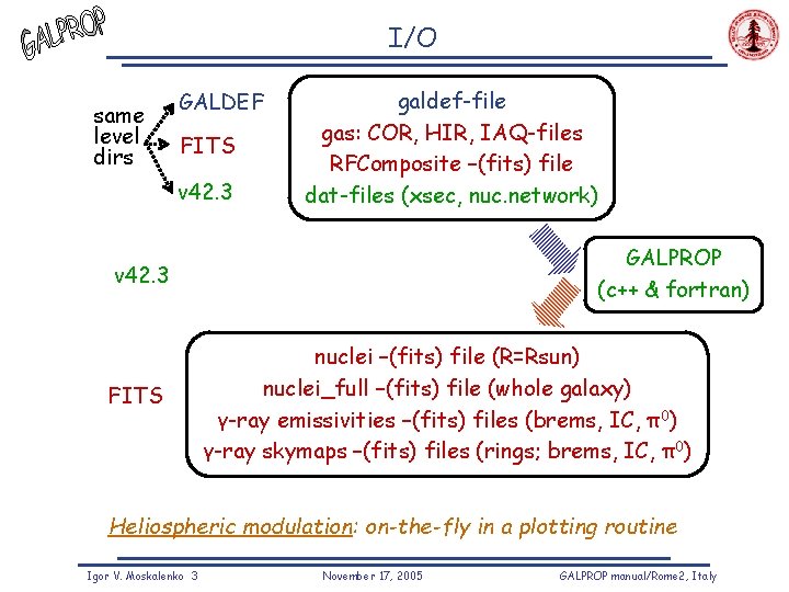
I/O same level dirs GALDEF FITS v 42. 3 galdef-file gas: COR, HIR, IAQ-files RFComposite –(fits) file dat-files (xsec, nuc. network) GALPROP (c++ & fortran) v 42. 3 FITS nuclei –(fits) file (R=Rsun) nuclei_full –(fits) file (whole galaxy) γ-ray emissivities –(fits) files (brems, IC, π0) γ-ray skymaps –(fits) files (rings; brems, IC, π0) Heliospheric modulation: on-the-fly in a plotting routine Igor V. Moskalenko 3 November 17, 2005 GALPROP manual/Rome 2, Italy

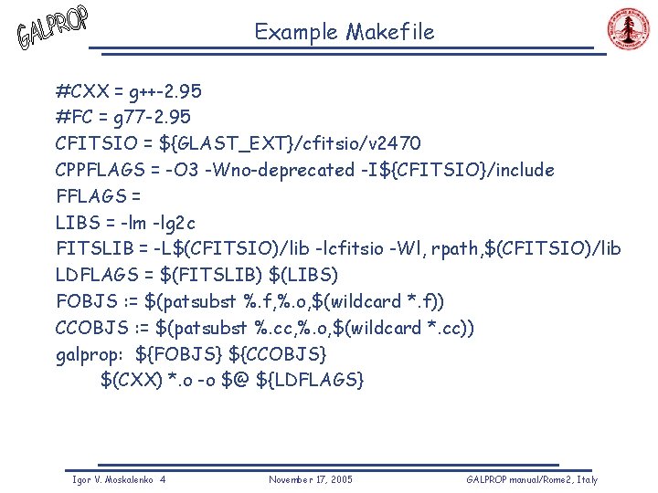
Example Makefile #CXX = g++-2. 95 #FC = g 77 -2. 95 CFITSIO = ${GLAST_EXT}/cfitsio/v 2470 CPPFLAGS = -O 3 -Wno-deprecated -I${CFITSIO}/include FFLAGS = LIBS = -lm -lg 2 c FITSLIB = -L$(CFITSIO)/lib -lcfitsio -Wl, rpath, $(CFITSIO)/lib LDFLAGS = $(FITSLIB) $(LIBS) FOBJS : = $(patsubst %. f, %. o, $(wildcard *. f)) CCOBJS : = $(patsubst %. cc, %. o, $(wildcard *. cc)) galprop: ${FOBJS} ${CCOBJS} $(CXX) *. o -o $@ ${LDFLAGS} Igor V. Moskalenko 4 November 17, 2005 GALPROP manual/Rome 2, Italy

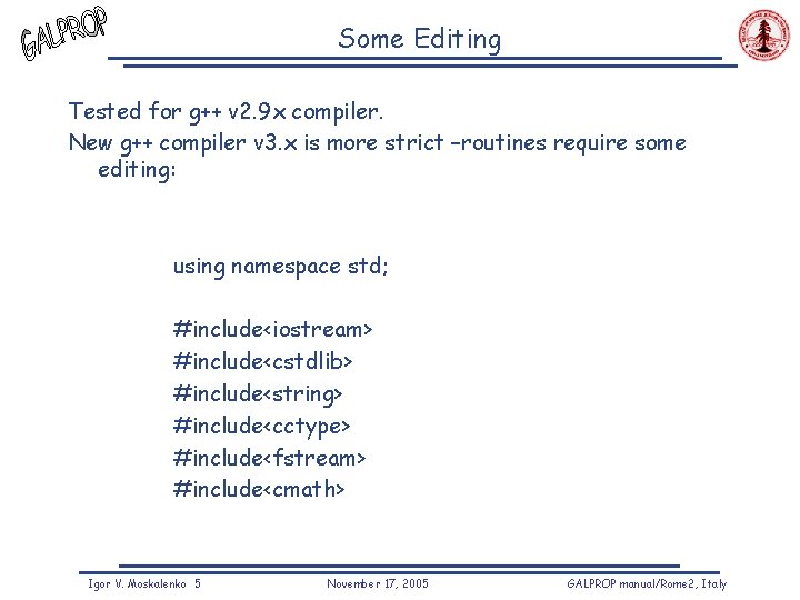
Some Editing Tested for g++ v 2. 9 x compiler. New g++ compiler v 3. x is more strict –routines require some editing: using namespace std; #include<iostream> #include<cstdlib> #include<string> #include<cctype> #include<fstream> #include<cmath> Igor V. Moskalenko 5 November 17, 2005 GALPROP manual/Rome 2, Italy

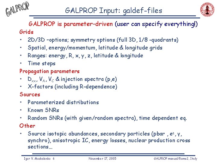
GALPROP Input: galdef-files GALPROP is parameter-driven (user can specify everything!) Grids • 2 D/3 D –options; symmetry options (full 3 D, 1/8 -quadrants) • Spatial, energy/momentum, latitude & longitude grids • Ranges: energy, R, x, y, z, latitude & longitude • Time steps Propagation parameters • Dxx, VA, VC & injection spectra (p, e) • X-factors (including R-dependence) Sources • Parameterized distributions • Known SNRs • Random SNRs (with given/random spectra), time dependent eq. Other • Source isotopic abundances, secondary particles (pbar , e±, γ, synchro), anisotropic IC, energy losses, nuclear production cross sections… Igor V. Moskalenko 6 November 17, 2005 GALPROP manual/Rome 2, Italy

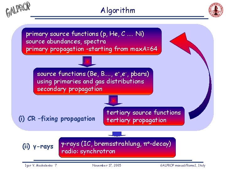
Algorithm primary source functions (p, He, C. . Ni) source abundances, spectra primary propagation -starting from max. A=64 source functions (Be, B. . , e+, e-, pbars) using primaries and gas distributions secondary propagation (i) CR –fixing propagation (ii) γ-rays Igor V. Moskalenko 7 tertiary source functions tertiary propagation -rays (IC, bremsstrahlung, πo-decay) radio: synchrotron November 17, 2005 GALPROP manual/Rome 2, Italy

GALPROP Output/FITS files Provides literally everything: • All nuclei and particle spectra in every grid point (x, y, R, z, E) -FITS files Separately for π0 -decay, IC, bremsstrahlung: • Emissivities in every grid point (x, y, R, z, E, process) • Skymaps with a given resolution (l, b, E, process) • Output of maps separated into HI, H 2, and rings to allow fitting X, metallicity gradient etc. Igor V. Moskalenko 8 November 17, 2005 GALPROP manual/Rome 2, Italy

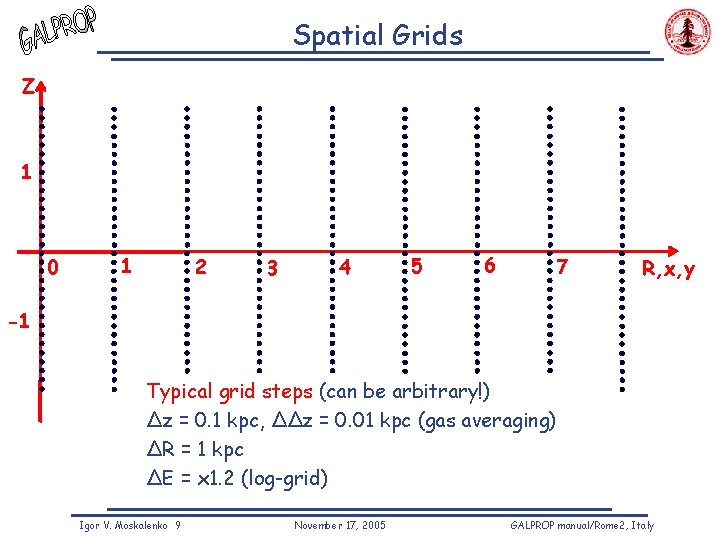
Spatial Grids Z 1 0 1 2 3 4 5 6 7 R, x, y -1 Typical grid steps (can be arbitrary!) Δz = 0. 1 kpc, ΔΔz = 0. 01 kpc (gas averaging) ΔR = 1 kpc ΔE = x 1. 2 (log-grid) Igor V. Moskalenko 9 November 17, 2005 GALPROP manual/Rome 2, Italy

GALPROP Calculations Constraints • Bin size (x, y, z) depends on the computer speed, RAM; final run can be done on a very fine grid ! • No other constraints ! –any required process/formalism can be implemented Calculations (γ -ray related) ØVectorization options Ø Now 64 bit to allow unlimited arrays Ø Heliospheric modulation: routinely force-field, more sophisticated model ? 1. For a given propagation parameters: propagate p, e, nuclei, secondaries (currently in 2 D) 2. The propagated distributions are stored 3. With propagated spectra: calculate the emissivities (π0 -decay, IC, bremss) in every grid point 4. Integrate the emissivities over the line of sight: • GALPROP has a full 3 D grid, but currently only 2 D gas maps (H 2, H II) • Using actual annular maps (column density) at the final step • High latitudes above b=40˚ -using integrated H I distribution Igor V. Moskalenko 10 November 17, 2005 GALPROP manual/Rome 2, Italy

Dark Matter in GALPROP DM annihilation products: χ0χ0−> p, pbar, e+, e−, γ A set of routines (gen_DM_source. cc) to assign • The DM density profile (NFW, isothermal etc. ) • Source functions for p, pbar, e+, e− • Source function for γ’s • A set of user-defined parameters (10 int, 10 double precision) in galdef-file Ø DM annihilation products particles are propagated in the same model as CR particles. Ø Calculation of skymaps for DM γ-rays Igor V. Moskalenko 11 November 17, 2005 GALPROP manual/Rome 2, Italy

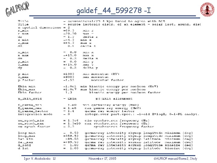
galdef_44_599278 -I Igor V. Moskalenko 12 November 17, 2005 GALPROP manual/Rome 2, Italy

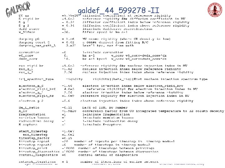
galdef_44_599278 -II Igor V. Moskalenko 13 November 17, 2005 GALPROP manual/Rome 2, Italy

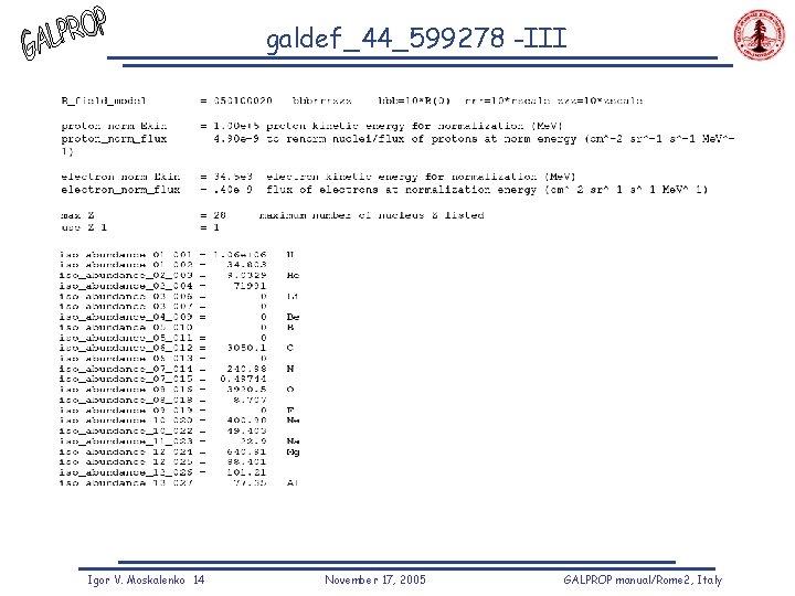
galdef_44_599278 -III Igor V. Moskalenko 14 November 17, 2005 GALPROP manual/Rome 2, Italy

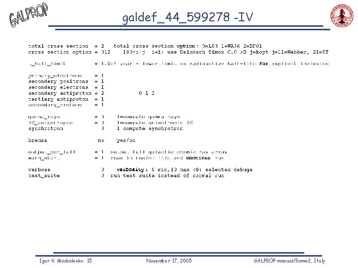
galdef_44_599278 -IV Igor V. Moskalenko 15 November 17, 2005 GALPROP manual/Rome 2, Italy

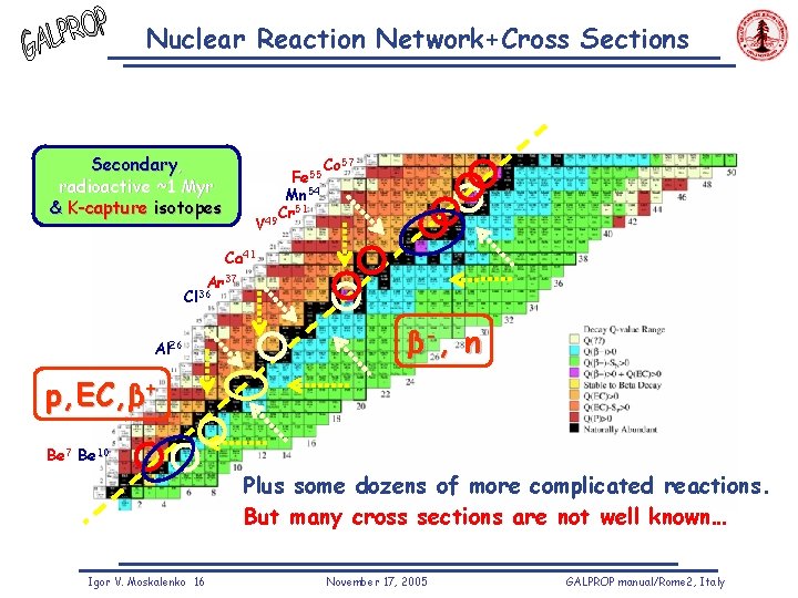
Nuclear Reaction Network+Cross Sections Secondary, radioactive ~1 Myr & K-capture isotopes Fe 55 V Co 57 Mn 54 Cr 51 49 Ca 41 Ar 37 Cl 36 Al 26 β -, n p, EC, β+ Be 7 Be 10 Plus some dozens of more complicated reactions. But many cross sections are not well known… Igor V. Moskalenko 16 November 17, 2005 GALPROP manual/Rome 2, Italy

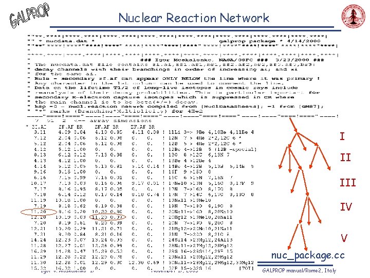
Nuclear Reaction Network I II IV V nuc_package. cc Igor V. Moskalenko 17 November 17, 2005 GALPROP manual/Rome 2, Italy

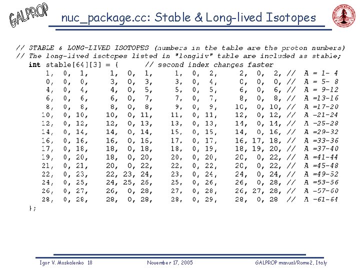
nuc_package. cc: Stable & Long-lived Isotopes Igor V. Moskalenko 18 November 17, 2005 GALPROP manual/Rome 2, Italy

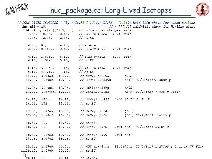
nuc_package. cc: Long-Lived Isotopes Igor V. Moskalenko 19 November 17, 2005 GALPROP manual/Rome 2, Italy

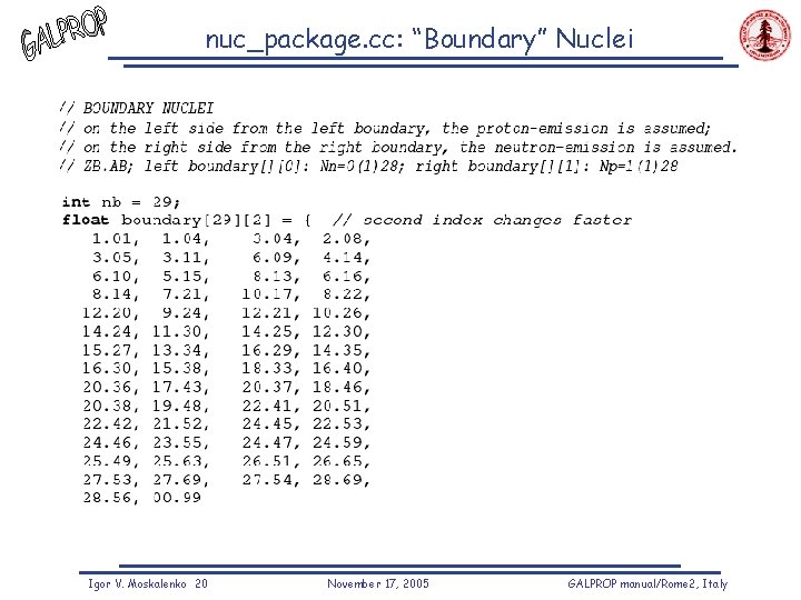
nuc_package. cc: “Boundary” Nuclei Igor V. Moskalenko 20 November 17, 2005 GALPROP manual/Rome 2, Italy

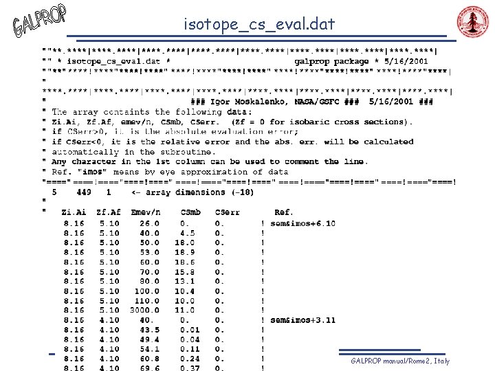
isotope_cs_eval. dat Igor V. Moskalenko 21 November 17, 2005 GALPROP manual/Rome 2, Italy

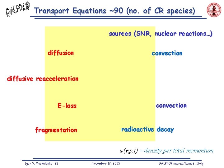
Transport Equations ~90 (no. of CR species) sources (SNR, nuclear reactions…) diffusion convection diffusive reacceleration convection E-loss radioactive decay fragmentation ψ(r, p, t) – density per total momentum Igor V. Moskalenko 22 November 17, 2005 GALPROP manual/Rome 2, Italy

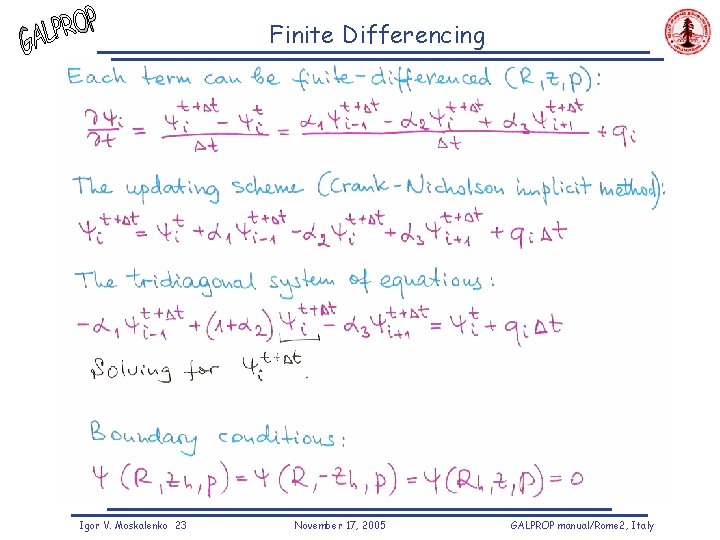
Finite Differencing Igor V. Moskalenko 23 November 17, 2005 GALPROP manual/Rome 2, Italy

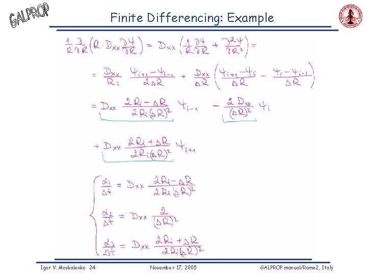
Finite Differencing: Example Igor V. Moskalenko 24 November 17, 2005 GALPROP manual/Rome 2, Italy

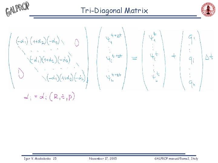
Tri-Diagonal Matrix Igor V. Moskalenko 25 November 17, 2005 GALPROP manual/Rome 2, Italy

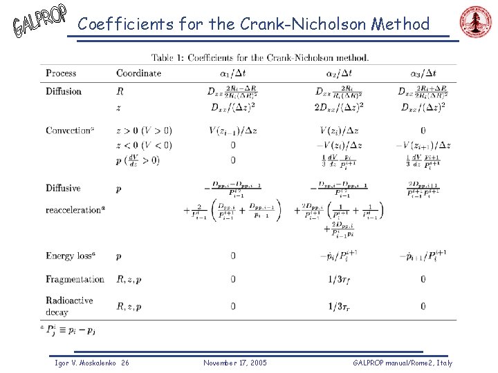
Coefficients for the Crank-Nicholson Method Igor V. Moskalenko 26 November 17, 2005 GALPROP manual/Rome 2, Italy

Near Future Developments Full 3 D Galactic structure: • 3 D gas maps (from S. Digel, S. Hunter and/or smbd else) • 3 D interstellar radiation & magnetic fields (A. Strong & T. Porter) Cross sections: • Blattnig et al. formalism for π0 -production • Diffractive dissociation with scaling violation (T. Kamae –param. ) • Isotopic cross sections (with S. Mashnik, LANL; try to motivate BNL, JENDL-Japan, other Nuc. Data Centers) Modeling the local structure: • Local SNRs with known positions and ages • Local Bubble, local clouds –may be done at the final calculation step (grid bin size ? ? ) Energy range: • Extend toward sub-Me. V range to compare with INTEGRAL diffuse emission (continuum; 511 ke. V line) Heliospheric modulation: • Implementing a modern formalism (Potgieter, Zank etc. ) Visualization tool (started) using the classes of CERN ROOT package: images, profiles, and spectra from GALPROP to be directly compared with data Improving the GALPROP module structure (for DM studies) Igor V. Moskalenko 27 November 17, 2005 GALPROP manual/Rome 2, Italy

More developments Ø Point sources: develop algorithm(s) for modeling the background and interface to the rest of GLAST software Ø Instrumental response: how to implement Ø Diffuse emission analysis has to include point source catalog! Ø At least, two diffuse models: with/without the “excess” Ø Develop test case(s) to test the accuracy of the numerical model (simple gas distribution, no energy losses, uniform ISRF etc. ) Ø Complete C++ package: rewrite several fortran routines in C++ Ø Develop a fitting procedure to make automatic fitting to B/C ratio, CR spectra and abundances Ø Develop a dedicated Web-site: – Controlled changes in GALPROP: tests +documentation +… – Allow for communication with users – Post relevant information: best models, gas maps, ISRF, nuclear cross sections… – Ability to run GALPROP on-line… Igor V. Moskalenko 28 November 17, 2005 GALPROP manual/Rome 2, Italy

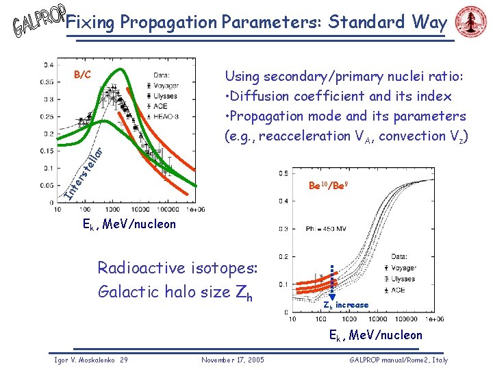
Fixing Propagation Parameters: Standard Way Using secondary/primary nuclei ratio: • Diffusion coefficient and its index • Propagation mode and its parameters (e. g. , reacceleration VA, convection Vz) te r st e lla r B/C In Be 10/Be 9 Ek, Me. V/nucleon Radioactive isotopes: Galactic halo size Zh Zh increase Ek, Me. V/nucleon Igor V. Moskalenko 29 November 17, 2005 GALPROP manual/Rome 2, Italy

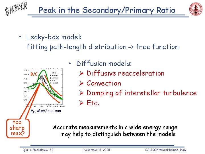
Peak in the Secondary/Primary Ratio • Leaky-box model: fitting path-length distribution -> free function • Diffusion models: Ø Diffusive reacceleration Ø Convection Ø Damping of interstellar turbulence Ø Etc. B/C Ek, Me. V/nucleon too sharp max? Accurate measurements in a wide energy range may help to distinguish between the models Igor V. Moskalenko 30 November 17, 2005 GALPROP manual/Rome 2, Italy

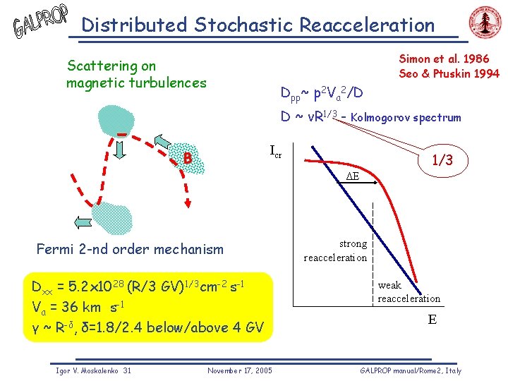
Distributed Stochastic Reacceleration Simon et al. 1986 Seo & Ptuskin 1994 Scattering on magnetic turbulences Dpp~ p 2 Va 2/D D ~ v. R 1/3 - Kolmogorov spectrum Icr B 1/3 ΔE Fermi 2 -nd order mechanism Dxx = 5. 2 x 1028 (R/3 GV)1/3 cm-2 s-1 Va = 36 km s-1 γ ~ R-δ, δ=1. 8/2. 4 below/above 4 GV Igor V. Moskalenko 31 November 17, 2005 strong reacceleration weak reacceleration E GALPROP manual/Rome 2, Italy

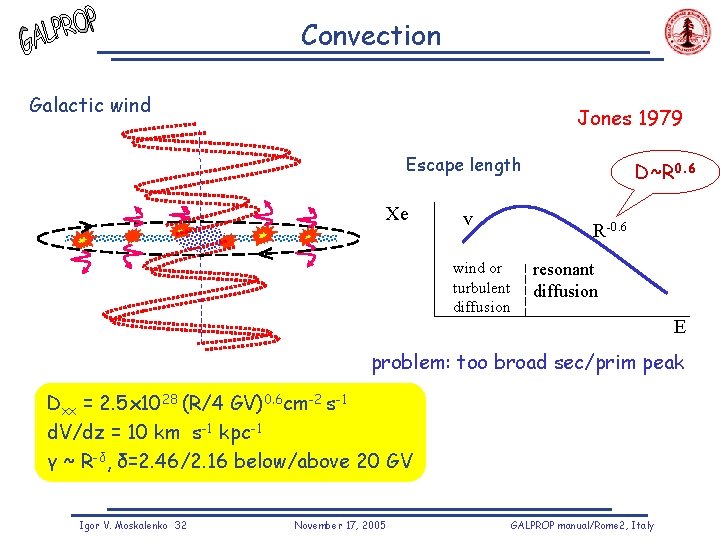
Convection Galactic wind Jones 1979 Escape length Xe v wind or turbulent diffusion D~R 0. 6 R-0. 6 resonant diffusion E problem: too broad sec/prim peak Dxx = 2. 5 x 1028 (R/4 GV)0. 6 cm-2 s-1 d. V/dz = 10 km s-1 kpc-1 γ ~ R-δ, δ=2. 46/2. 16 below/above 20 GV Igor V. Moskalenko 32 November 17, 2005 GALPROP manual/Rome 2, Italy

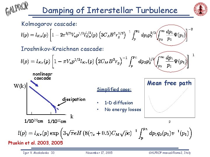
Damping of Interstellar Turbulence Kolmogorov cascade: Iroshnikov-Kraichnan cascade: nonlinear cascade W(k) Simplified case: dissipation 1/1020 cm 1/1012 cm • • Mean free path 1 -D diffusion No energy losses k Ptuskin et al. 2003, 2005 Igor V. Moskalenko 33 November 17, 2005 GALPROP manual/Rome 2, Italy

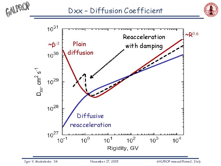
Dxx – Diffusion Coefficient ~β-3 Plain diffusion Reacceleration with damping ~R 0. 6 Diffusive reacceleration Igor V. Moskalenko 34 November 17, 2005 GALPROP manual/Rome 2, Italy

How It Is Really Done: Secondary Particles • Positrons/electrons p+p->π, K->e± (MS 1998) – Dermer 1986 method: LE –Stecker Δ-isobar model (isotropic decay), HE –scaling (inv. x-section: Stephens & Badhwar 1981), plus interpolation in between – Pion decay “includes” polarization of muons – Kaon decay – scaling (Stephens & Badhwar 1981) • Antiprotons (M et al. 2002) – pp Inclusive production x-section (Tan & Ng 1983) – p. A, AA-> pbar –scaling using Gaisser & Schaeffer 1992 or Simon et al. 1998 –results similar – Total inelastic x-section (p: TN’ 83, A: Moiseev & Ormes 1997) – p+pbar annihilation x-section = (p+pbar)tot – (p+p)tot (LE: TN’ 83, HE: PDG’ 00 –Regge parameterization) Igor V. Moskalenko 35 November 17, 2005 GALPROP manual/Rome 2, Italy

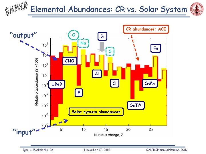
Elemental Abundances: CR vs. Solar System CR abundances: ACE “output” O Si Na Fe S CNO Al Cl Li. Be. B Cr. Mn F Sc. Ti. V Solar system abundances “input” Igor V. Moskalenko 36 November 17, 2005 GALPROP manual/Rome 2, Italy

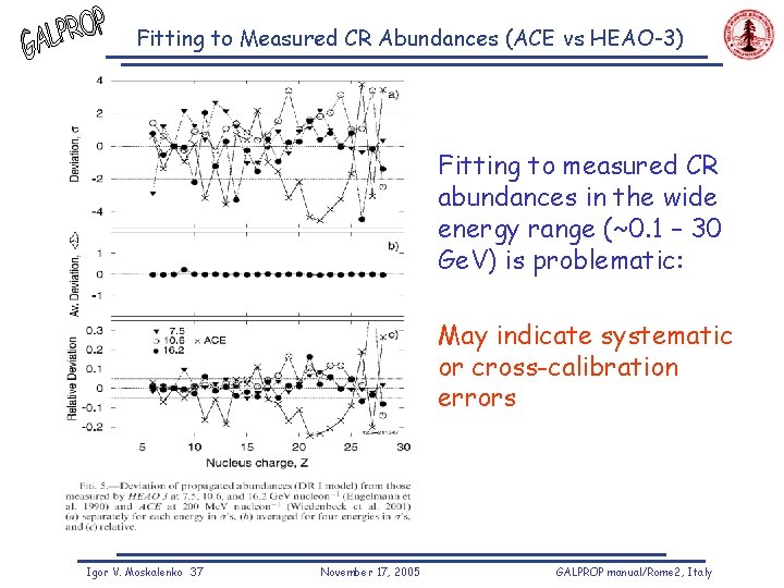
Fitting to Measured CR Abundances (ACE vs HEAO-3) Fitting to measured CR abundances in the wide energy range (~0. 1 – 30 Ge. V) is problematic: May indicate systematic or cross-calibration errors Igor V. Moskalenko 37 November 17, 2005 GALPROP manual/Rome 2, Italy

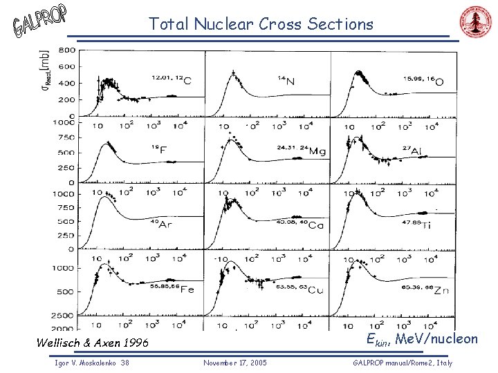
Total Nuclear Cross Sections Ekin, Me. V/nucleon Wellisch & Axen 1996 Igor V. Moskalenko 38 November 17, 2005 GALPROP manual/Rome 2, Italy

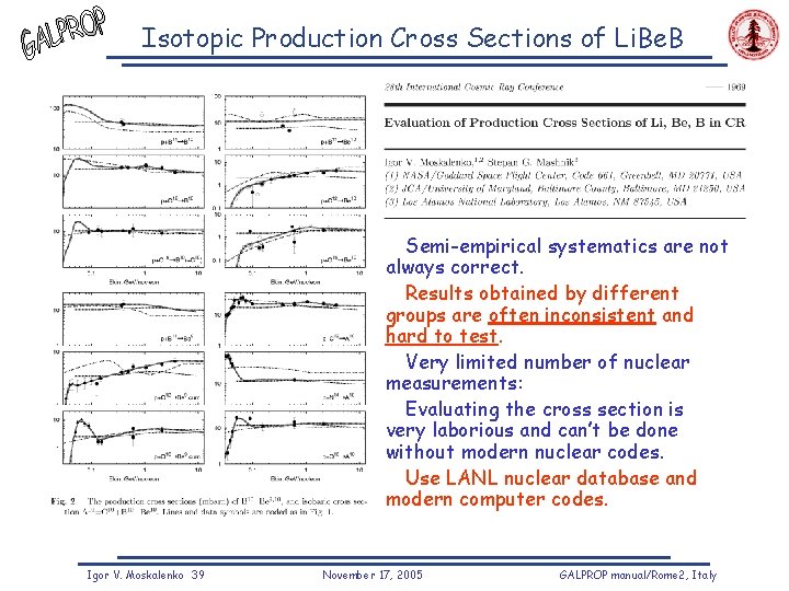
Isotopic Production Cross Sections of Li. Be. B Semi-empirical systematics are not always correct. Results obtained by different groups are often inconsistent and hard to test. Very limited number of nuclear measurements: Evaluating the cross section is very laborious and can’t be done without modern nuclear codes. Use LANL nuclear database and modern computer codes. Igor V. Moskalenko 39 November 17, 2005 GALPROP manual/Rome 2, Italy

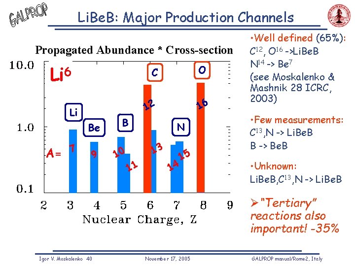
Li. Be. B: Major Production Channels Propagated Abundance * Cross-section Li 6 Li Be A= 7 9 C O 12 16 B 10 N 13 11 14 15 • Well defined (65%): C 12, O 16 ->Li. Be. B N 14 -> Be 7 (see Moskalenko & Mashnik 28 ICRC, 2003) • Few measurements: C 13, N -> Li. Be. B B -> Be. B • Unknown: Li. Be. B, C 13, N -> Li. Be. B Ø“Tertiary” reactions also important! -35% Igor V. Moskalenko 40 November 17, 2005 GALPROP manual/Rome 2, Italy

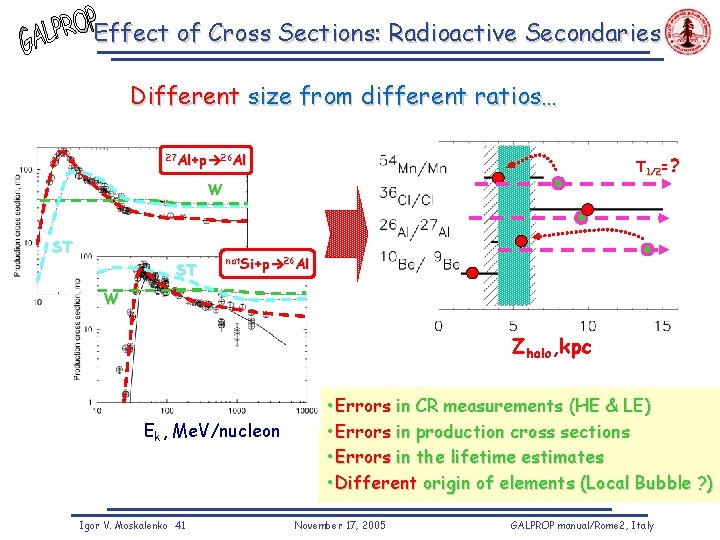
Effect of Cross Sections: Radioactive Secondaries Different size from different ratios… 27 Al+p 26 Al T 1/2=? W ST ST nat. Si+p 26 Al W Zhalo, kpc Ek, Me. V/nucleon Igor V. Moskalenko 41 • Errors in CR measurements (HE & LE) • Errors in production cross sections • Errors in the lifetime estimates • Different origin of elements (Local Bubble ? ) November 17, 2005 GALPROP manual/Rome 2, Italy

How It Is Really Done: Nucleons • • Calculated for p+A reactions and scaled for α+A (Ferrando et al. 1988) Calculation of total nuclear cross sections • Calculation of isotopic production cross sections • Nuclear reaction network – Letaw et al. 1983 – Wellisch & Axen 1996 (corrected), Z>5 – Barashenkov & Polanski 2001 – Webber et al. 1993 (non-renormalized, renormalized); E>200 Me. V/nucleon, essentially flat – Silberberg & Tsao 2000 (non-renormalized, renormalized); claim that it works at all energies, but is problematic sometimes – Fits to the available data (LANL, Webber et al. , etc. ) in the form of a function or a table (see. dat files), but data may not be always available – Use the best of all three, but very time consuming work – Nuclear Data Tables (includes several decay channels + branching) – Standard β± -decay, emission of p, n – K-capture isotopes can be treated separately Igor V. Moskalenko 42 November 17, 2005 GALPROP manual/Rome 2, Italy

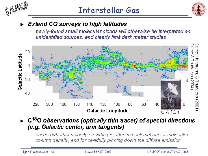
Interstellar Gas ► Extend CO surveys to high latitudes – newly-found small molecular clouds will otherwise be interpreted as 20 0 -20 -40 220 200 180 160 140 120 100 80 Galactic Longitude ► 60 40 20 0 Cf. A 1. 2 m Dame, Hartmann, & Thaddeus (2001) Dame & Thaddeus (2004) Galactic Latitude unidentified sources, and clearly limit dark matter studies C 18 O observations (optically thin tracer) of special directions (e. g. Galactic center, arm tangents) – assess whether velocity crowding is affecting calculations of molecular column density, and for carefully pinning down the diffuse emission Igor V. Moskalenko 43 November 17, 2005 GALPROP manual/Rome 2, Italy

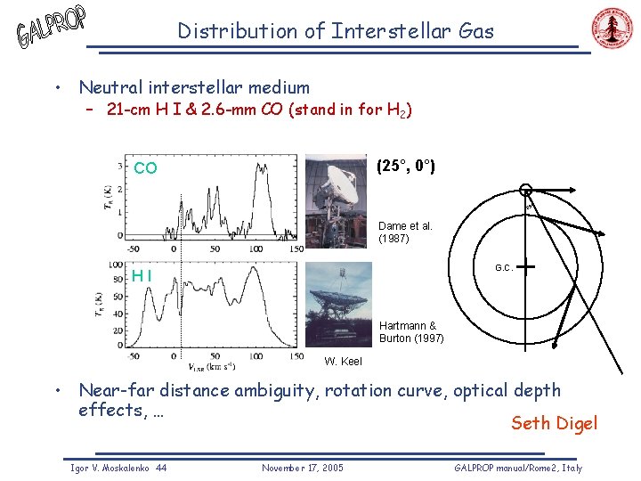
Distribution of Interstellar Gas • Neutral interstellar medium – 21 -cm H I & 2. 6 -mm CO (stand in for H 2) (25°, 0°) CO 25° Dame et al. (1987) G. C. HI Hartmann & Burton (1997) W. Keel • Near-far distance ambiguity, rotation curve, optical depth effects, … Seth Digel Igor V. Moskalenko 44 November 17, 2005 GALPROP manual/Rome 2, Italy

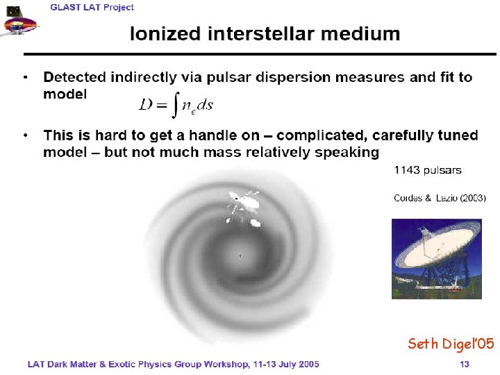
Seth Digel’ 05 Igor V. Moskalenko 45 November 17, 2005 GALPROP manual/Rome 2, Italy

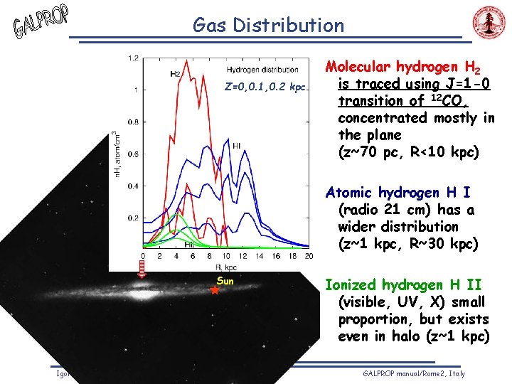
Gas Distribution Z=0, 0. 1, 0. 2 kpc Molecular hydrogen H 2 is traced using J=1 -0 transition of 12 CO, concentrated mostly in the plane (z~70 pc, R<10 kpc) Atomic hydrogen H I (radio 21 cm) has a wider distribution (z~1 kpc, R~30 kpc) Sun Igor V. Moskalenko 46 November 17, 2005 Ionized hydrogen H II (visible, UV, X) small proportion, but exists even in halo (z~1 kpc) GALPROP manual/Rome 2, Italy

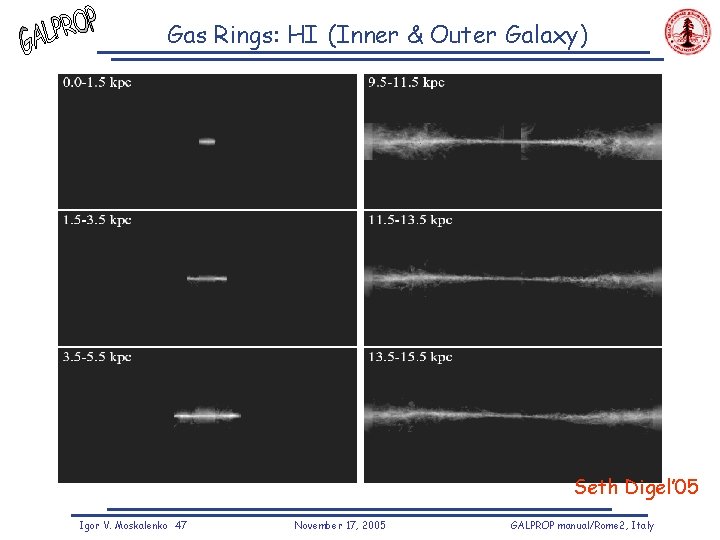
Gas Rings: HI (Inner & Outer Galaxy) Seth Digel’ 05 Igor V. Moskalenko 47 November 17, 2005 GALPROP manual/Rome 2, Italy

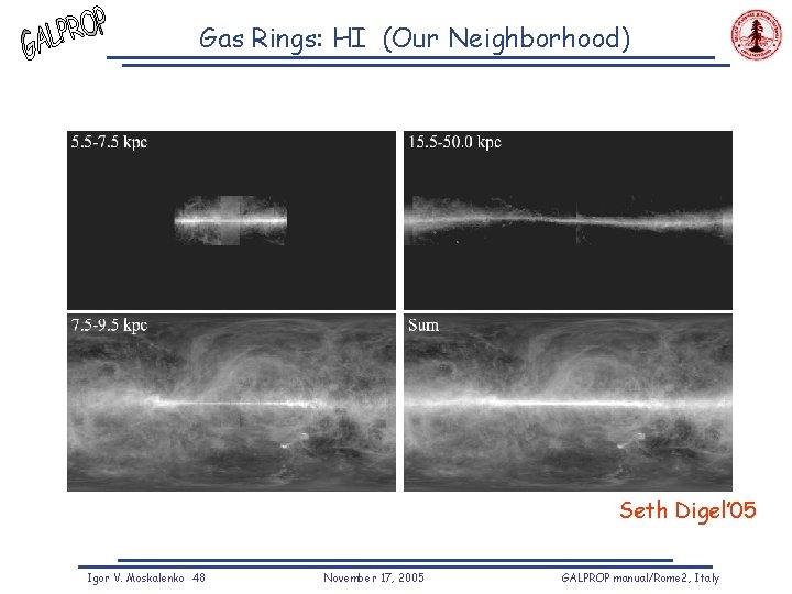
Gas Rings: HI (Our Neighborhood) Seth Digel’ 05 Igor V. Moskalenko 48 November 17, 2005 GALPROP manual/Rome 2, Italy

How It Is Really Done: Gammas • Bremsstrahlung (Koch & Motz 1959, SMR 2000) –many different regimes: – LE: 0. 01 < Ekin < 0. 07 Me. V –nonrelativistic non-screened brems – Intermediate: 0. 07 < Ekin <2 Me. V – HE: Ekin > 2 Me. V arbitrary screening: unshielded charge, 1 -, 2 electron atoms (form factors, Hylleraas, Hertree-Fock wave functions) – Fano-Sauter limit: k->Ekin • “Anisotropic” IC (MS 2000) – Takes into account the anisotropic angular distribution of background photons • Neutral pion decay (see “secondary positrons/electrons”) • Synchrotron radiation (Ginzburg 1979, Ghisellini et al. 1988) – Averaging over pitch angle – Uses total magnetic field (regular + random) • Emissivities: uses “real” H 2, H I gas column densities (“rings”) • Skymap calculations: integration over the line of sight Igor V. Moskalenko 49 November 17, 2005 GALPROP manual/Rome 2, Italy

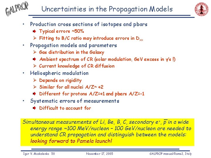
Uncertainties in the Propagation Models • • Production cross sections of isotopes and pbars Typical errors ~50% Ø Fitting to B/C ratio may introduce errors in Dxx Propagation models and parameters Ø Gas distribution in the Galaxy Ambient spectrum of CR (solar modulation, Ge. V excess in γ’s !) Ø Current knowledge of CR diffusion • Heliospheric modulation Ø Depends on rigidity Ø Similar for all nuclei A/Z~ +2 Different for protons A/Z=+1 and pbars A/Z=-1 • Systematic errors of measurements Difficult to account for e +, _ Simultaneous measurements of Li, Be, B, C, secondary p in a wide energy range ~100 Me. V/nucleon – 100 Ge. V/nucleon are needed to understand CR propagation and distinguish between the models: looking forward to Pamela launch! Igor V. Moskalenko 50 November 17, 2005 GALPROP manual/Rome 2, Italy